Analysis of the Wuidart et al. mouse single-cell RNA-seq data
Tobias Tekath
2021-11-18
Source:vignettes/Wuidart_mouse_single-cell_analysis.Rmd
Wuidart_mouse_single-cell_analysis.RmdThis vignette exemplifies the analysis of single-cell RNA-seq data with DTUrtle. The data used in this vignette is publicly available as Bioproject PRJNA433520 and the used FASTQ-files can be downloaded from here. The corresponding publication from Wuidart et al. can be found here.
The following code shows an example of an DTUrtle workflow. Assume we have performed the pre-processing as described here and the R working directory is a newly created folder called dtu_results.
Setup
Load the DTUrtle package and set the BiocParallel parameter. It is recommended to perform computations in parallel, if possible.
library(DTUrtle)
#> Loading required package: sparseDRIMSeq
#> To cite DTUrtle in publications use:
#>
#>  Tobias Tekath, Martin Dugas.
#>  Differential transcript usage analysis
#>  of bulk and single-cell RNA-seq data with DTUrtle.
#>  Bioinformatics,
#>  2021.
#>  https://doi.org/10.1093/bioinformatics/btab629.
#>
#> Use citation(DTUrtle) for BibTeX information.
#use up to 10 cores for computation
biocpar <- BiocParallel::MulticoreParam(10)
Import and format data
We want to start by reading-in our quantification counts, as well as a file specifying which transcript ID or name belongs to which gene ID or name.
Importing and processing GTF annotation (tx2gene)
To get this transcript to gene (tx2gene) mapping, we will utilize the already present Gencode annotation file gencode.vM24.annotation_spike.gtf. The import_gtf() function utilizes the a rtracklayer package and returns a transcript-level filtered version of the available data.
tx2gene <- import_gtf(gtf_file = "../gencode.vM24.annotation_spike.gtf")
head(tx2gene, n=3)
#>   seqnames   start     end width strand  source       type score phase
#> 1     chr1 3073253 3074322  1070      +  HAVANA transcript    NA    NA
#> 2     chr1 3102016 3102125   110      + ENSEMBL transcript    NA    NA
#> 3     chr1 3205901 3216344 10444      -  HAVANA transcript    NA    NA
#>                gene_id        transcript_id      gene_type     gene_name
#> 1 ENSMUSG00000102693.1 ENSMUST00000193812.1            TEC 4933401J01Rik
#> 2 ENSMUSG00000064842.1 ENSMUST00000082908.1          snRNA       Gm26206
#> 3 ENSMUSG00000051951.5 ENSMUST00000162897.1 protein_coding          Xkr4
#>        transcript_type   transcript_name level transcript_support_level
#> 1                  TEC 4933401J01Rik-201     2                       NA
#> 2                snRNA       Gm26206-201     3                       NA
#> 3 processed_transcript          Xkr4-203     2                        1
#>        mgi_id   tag          havana_gene    havana_transcript protein_id ccdsid
#> 1 MGI:1918292 basic OTTMUSG00000049935.1 OTTMUST00000127109.1       <NA>   <NA>
#> 2 MGI:5455983 basic                 <NA>                 <NA>       <NA>   <NA>
#> 3 MGI:3528744  <NA> OTTMUSG00000026353.2 OTTMUST00000086625.1       <NA>   <NA>
#>    ont
#> 1 <NA>
#> 2 <NA>
#> 3 <NA>
This tx2gene file does not contain the manually added ERCC spike-in sequences, as these are marked as exon in the corresponding ERCC GTF-file. Thus we will add these ERCC sequences again to the annotation:
#set featrue_type=NULL to not filter the GTF
ercc_gtf <- import_gtf(gtf_file = "../ERCC92.gtf", feature_type = NULL)
#change not necessary transcript-IDs
ercc_gtf$transcript_id <- ercc_gtf$gene_id

tx2gene <- merge(tx2gene, ercc_gtf, all = TRUE)

#fix missing gene_name and transcript_name for ERCCs
tx2gene$gene_name[is.na(tx2gene$gene_name)] <- tx2gene$gene_id[is.na(tx2gene$gene_name)]
tx2gene$transcript_name[is.na(tx2gene$transcript_name)] <- tx2gene$transcript_id[is.na(tx2gene$transcript_name)]
There are a lot of columns present in the data frame, but at the moment we are mainly interested in the columns gene_id, gene_name, transcript_id and transcript_name.
As we want to use gene and transcript names as the main identifiers in our analysis (so we can directly say: Gene x is differential), we should ensure that each gene / transcript name maps only to a single gene / transcript id.
For this we can use the DTUrtle function one_to_one_mapping(), which checks if there are identifiers, which relate to the same name. If this is the case, the names (not the identifiers) are slightly altered by appending a number. If id_x and id_y both have the name ABC, the id_y name is altered to ABC_2 by default.
tx2gene$gene_name <- one_to_one_mapping(name = tx2gene$gene_name, id = tx2gene$gene_id)
#> Changed 109 names.
tx2gene$transcript_name <- one_to_one_mapping(name = tx2gene$transcript_name, id = tx2gene$transcript_id)
#> No changes needed -> already one to one mapping.
We see that it was a good idea to ensure the one to one mapping for gene names, as 109 doublets have been corrected.
For the run_drimseq() tx2gene parameter, we need a data frame, where the first column specifies the transcript identifiers and the second column specifying the corresponding gene names. Rather than subsetting the data frame, a column reordering is proposed, so that additional data can still be used in further steps. DTUrtle makes sure to carry over additional data columns in the analysis steps. To reorder the columns of our tx2gene data frame, we can utilize the move_columns_to_front() functionality.
tx2gene <- move_columns_to_front(df = tx2gene, columns = c("transcript_name", "gene_name"))
head(tx2gene, n=5)
#>     transcript_name     gene_name seqnames   start     end  width strand
#> 1 4933401J01Rik-201 4933401J01Rik     chr1 3073253 3074322   1070      +
#> 2       Gm26206-201       Gm26206     chr1 3102016 3102125    110      +
#> 3          Xkr4-203          Xkr4     chr1 3205901 3216344  10444      -
#> 4          Xkr4-202          Xkr4     chr1 3206523 3215632   9110      -
#> 5          Xkr4-201          Xkr4     chr1 3214482 3671498 457017      -
#>    source       type score phase              gene_id        transcript_id
#> 1  HAVANA transcript    NA    NA ENSMUSG00000102693.1 ENSMUST00000193812.1
#> 2 ENSEMBL transcript    NA    NA ENSMUSG00000064842.1 ENSMUST00000082908.1
#> 3  HAVANA transcript    NA    NA ENSMUSG00000051951.5 ENSMUST00000162897.1
#> 4  HAVANA transcript    NA    NA ENSMUSG00000051951.5 ENSMUST00000159265.1
#> 5  HAVANA transcript    NA    NA ENSMUSG00000051951.5 ENSMUST00000070533.4
#>        gene_type      transcript_type level transcript_support_level
#> 1            TEC                  TEC     2                       NA
#> 2          snRNA                snRNA     3                       NA
#> 3 protein_coding processed_transcript     2                        1
#> 4 protein_coding processed_transcript     2                        1
#> 5 protein_coding       protein_coding     2                        1
#>        mgi_id   tag          havana_gene    havana_transcript
#> 1 MGI:1918292 basic OTTMUSG00000049935.1 OTTMUST00000127109.1
#> 2 MGI:5455983 basic                 <NA>                 <NA>
#> 3 MGI:3528744  <NA> OTTMUSG00000026353.2 OTTMUST00000086625.1
#> 4 MGI:3528744  <NA> OTTMUSG00000026353.2 OTTMUST00000086624.1
#> 5 MGI:3528744  CCDS OTTMUSG00000026353.2 OTTMUST00000065166.1
#>             protein_id      ccdsid  ont
#> 1                 <NA>        <NA> <NA>
#> 2                 <NA>        <NA> <NA>
#> 3                 <NA>        <NA> <NA>
#> 4                 <NA>        <NA> <NA>
#> 5 ENSMUSP00000070648.4 CCDS14803.1 <NA>
This concludes the tx2gene formatting.
Reading in quantification data
The read-in of the quantification counts can be achieved with import_counts(), which uses the tximport package in the background. This function is able to parse the output of many different quantification tools. Advanced users might be able to tune parameters to parse arbitrary output files from currently not supported tools.
In the pre-processing vignette we quantified the counts with Salmon. The folder structure of the quantification results folder looks like this:
head(list.files("../salmon/"))
#> [1] "index"      "multiqc"    "SRR6690781" "SRR6690782" "SRR6690783"
#> [6] "SRR6690784"
We will create a named files vector, pointing to the quant.sf file for each sample. The names help to differentiate the samples later on.
The files object looks like this:
#>                      SRR6690781                      SRR6690782
#> "../salmon/SRR6690781/quant.sf" "../salmon/SRR6690782/quant.sf"
#>                      SRR6690783                      SRR6690784
#> "../salmon/SRR6690783/quant.sf" "../salmon/SRR6690784/quant.sf"
#>                      SRR6690785                      SRR6690786
#> "../salmon/SRR6690785/quant.sf" "../salmon/SRR6690786/quant.sf"
The actual import will be performed with import_counts(). As we are analyzing bulk RNA-seq data, the raw counts should be scaled regarding transcript length and/or library size prior to analysis. DTUrtle will default to appropriate scaling schemes for your data. It is advised to provide a transcript to gene mapping for the tx2gene parameter, as then the tximport dtuScaledTPM scaling scheme can be applied. This schemes is especially designed for DTU analysis and scales by using the median transcript length among isoforms of a gene, and then the library size.
In contrast to many other single-cell protocols, Smart-seq2 creates full-length reads, i.e. the read fragments are not only originating from the 5’- or 3’-End of the mRNA. This is preferential for DTU analysis, but also implicates that the reads could be prone to some full-length specific biases (see DTUrtle publication for more details). Thus, as for standard bulk RNA-seq analysis, the dtuScaledTPM scaling scheme should be applied (in contrast for example for 3’- 10X Chromium reads).
The raw counts from Salmon are named in regard to the transcript_id, thus we will provide an appropriate tx2gene parameter here. Downstream we want to use the transcript_name rather than the transcript_id, so we change the row names of the counts:
cts <- import_counts(files, type = "salmon", tx2gene=tx2gene[,c("transcript_id", "gene_name")])
#> Reading in 384 salmon runs.
#> Using 'dtuScaledTPM' for 'countsFromAbundance'.
#> reading in files with read_tsv
#> 1 2 3 4 5 6 7 8 9 10 11 12 13 14 15 16 17 18 19 20 21 22 23 24 25 26 27 28 29 30 31 32 33 34 35 36 37 38 39 40 41 42 43 44 45 46 47 48 49 50 51 52 53 54 55 56 57 58 59 60 61 62 63 64 65 66 67 68 69 70 71 72 73 74 75 76 77 78 79 80 81 82 83 84 85 86 87 88 89 90 91 92 93 94 95 96 97 98 99 100 101 102 103 104 105 106 107 108 109 110 111 112 113 114 115 116 117 118 119 120 121 122 123 124 125 126 127 128 129 130 131 132 133 134 135 136 137 138 139 140 141 142 143 144 145 146 147 148 149 150 151 152 153 154 155 156 157 158 159 160 161 162 163 164 165 166 167 168 169 170 171 172 173 174 175 176 177 178 179 180 181 182 183 184 185 186 187 188 189 190 191 192 193 194 195 196 197 198 199 200 201 202 203 204 205 206 207 208 209 210 211 212 213 214 215 216 217 218 219 220 221 222 223 224 225 226 227 228 229 230 231 232 233 234 235 236 237 238 239 240 241 242 243 244 245 246 247 248 249 250 251 252 253 254 255 256 257 258 259 260 261 262 263 264 265 266 267 268 269 270 271 272 273 274 275 276 277 278 279 280 281 282 283 284 285 286 287 288 289 290 291 292 293 294 295 296 297 298 299 300 301 302 303 304 305 306 307 308 309 310 311 312 313 314 315 316 317 318 319 320 321 322 323 324 325 326 327 328 329 330 331 332 333 334 335 336 337 338 339 340 341 342 343 344 345 346 347 348 349 350 351 352 353 354 355 356 357 358 359 360 361 362 363 364 365 366 367 368 369 370 371 372 373 374 375 376 377 378 379 380 381 382 383 384
rownames(cts) <- tx2gene$transcript_name[match(rownames(cts), tx2gene$transcript_id)]
dim(cts)
#> [1] 141040    384
There are ~141k features left for the 384 samples/cells. Please note, that in contrast to the single-cell workflow utilizing combine_to_matrix(), these counts also include features with no expression. These will be filtered out by the DTUrtle filtering step in run_drimseq().
Sample metadata
Finally, we need a sample metadata data frame, specifying which sample belongs to which comparison group. This table is also convenient to store and carry over additional metadata.
We can reuse the ENA Bioproject report table from here:
pd <- read.table("../filereport_read_run_PRJNA433520_tsv.txt", sep = "\t", header = TRUE, stringsAsFactors = FALSE)

#especially the columns run_accession and sample_title are of interest
pd <- pd[,c("run_accession", "sample_title")]
head(pd, n=10)
#>    run_accession                                       sample_title
#> 1     SRR6690781            50 Cell Control Basal TAAGGCGA-CTCTCTAT
#> 2     SRR6690782          50 Cell Control Luminal CGTACTAG-CTCTCTAT
#> 3     SRR6690783                Single Basal Cell AGGCAGAA-CTCTCTAT
#> 4     SRR6690784                Single Basal Cell TCCTGAGC-CTCTCTAT
#> 5     SRR6690785                Single Basal Cell GGACTCCT-CTCTCTAT
#> 6     SRR6690786                Single Basal Cell TAGGCATG-CTCTCTAT
#> 7     SRR6690787 Single Embryonal Progenitor Cell CTCTCTAC-CTCTCTAT
#> 8     SRR6690788                Single Basal Cell CGAGGCTG-CTCTCTAT
#> 9     SRR6690789                Single Basal Cell AAGAGGCA-CTCTCTAT
#> 10    SRR6690790                Single Basal Cell GTAGAGGA-CTCTCTAT
We see, the first two samples are control samples consisting out of reads of 50 cells each, while the other samples are reads from a single cell. We can create a group assignment based on this information:
pd$group <- gsub("50 Cell |Single | [ATCG]{8}-[ATCG]{8}", "", pd$sample_title)
table(pd$group)
#>
#>                   Basal Cell                Control Basal
#>                          118                            1
#> Control Embryonal Progenitor              Control Luminal
#>                            1                            1
#>    Embryonal Progenitor Cell                 Luminal Cell
#>                          137                          122
#>             Negative Control
#>                            4
Cell filtering
We perform the same cell filtering as described in Wuidart et al., i.e. we exclude cells that have fewer than 10^5 counts, show expression of fewer than 2500 unique genes, have more than 20% counts belonging to ERCC sequences, or have more than 8% counts belonging to mitochondrial sequences.
#number of counts
pd$n_reads <- colSums(cts)[match(pd$run_accession, colnames(cts))]

#number of expressed genes --- summarize transcript level counts to gene level.
cts_gene <- summarize_to_gene(mtx = cts, tx2gene = tx2gene)
pd$unq_gene <- colSums(cts_gene!=0)[match(pd$run_accession, colnames(cts_gene))]

#proportion of ERCC counts
ercc_genes <-  rownames(cts)[startsWith(rownames(cts), "ERCC")]
pd$prop_ercc <- (colSums(cts[ercc_genes,])[match(pd$run_accession, colnames(cts))])/pd$n_reads

#proportion of MT counts
mt_genes <- unique(tx2gene$transcript_name[tx2gene$seqnames %in% c("chrM")])
pd$prop_MT <- (colSums(cts[mt_genes,])[match(pd$run_accession, colnames(cts))])/pd$n_reads

#create vector of cells not passing the filters.
excl_cells <- pd$run_accession[pd$n_reads<10^5|pd$unq_gene<2500|pd$prop_ercc>0.2|pd$prop_MT>0.08]
length(excl_cells)
#> [1] 108
Of the initial 384 cells, 108 are already on the exclude list because of these thresholds. In Wuidart et al. further constraints are placed: “BCs and EMPs that showed no expression of either K5 or K14, and LCs that did not express K8 were further excluded. Cells coming from a row F of the 384-well plate that showed systematic mixing of LC and BC markers were excluded from further analysis due to a likely pipetting error.”
‘K5’, ‘K14’ and ‘K8’ probably refer to the Keratin genes ‘Krt5’, ‘Krt14’ and ‘Krt8’, respectively. As the plate design of the experiment was not published, and therefore we do not know which cells where in row F, we try to impute the cells with mixed signals.
#get expression of Keratin genes 'Krt5', 'Krt14' and 'Krt8'
pd$krt5_expr <- colSums(cts_gene["Krt5",,drop=FALSE])[match(pd$run_accession, colnames(cts_gene))]
pd$krt14_expr <- colSums(cts_gene["Krt14",,drop=FALSE])[match(pd$run_accession, colnames(cts_gene))]
pd$krt8_expr <- colSums(cts_gene["Krt8",,drop=FALSE])[match(pd$run_accession, colnames(cts_gene))]

#we set a threshold of 1 count for 'expression'
excl_bc_emp <- pd$run_accession[pd$group %in% c("Basal Cell", "Embryonal Progenitor Cell") & (pd$krt5_expr<1 | pd$krt14_expr<1)]
excl_lc <- pd$run_accession[pd$group %in% c("Luminal Cell") & pd$krt8_expr<1]

#look how combined control samples express Keratin genes:
pd[startsWith(pd$group, "Control"),c("sample_title", "krt5_expr", "krt14_expr", "krt8_expr")]
#>                                              sample_title  krt5_expr krt14_expr
#> 1                 50 Cell Control Basal TAAGGCGA-CTCTCTAT 209.535321  1630.0407
#> 2               50 Cell Control Luminal CGTACTAG-CTCTCTAT   1.479728     0.0000
#> 25 50 Cell Control Embryonal Progenitor TAAGGCGA-TATCCTCT  68.929881   901.0704
#>    krt8_expr
#> 1   548.3311
#> 2  4859.8377
#> 25  255.6545

#exclude cells with krt5 & krt14 > 10 and krt8 > 1000
excl_mixed <- pd$run_accession[pd$group %in% c("Basal Cell", "Embryonal Progenitor Cell", "Luminal Cell") & (pd$krt5_expr>10 | pd$krt14_expr>10) & pd$krt8_expr>1000]
message(paste0("Exclude ",length(excl_mixed), " cells because of mixed signal."))
#> Exclude 31 cells because of mixed signal.

excl_cells <- unique(c(excl_cells, excl_bc_emp, excl_lc, excl_mixed))
length(excl_cells)
#> [1] 165
Combining all the given constraints, we have 165 cells on our exclude list. Thus, we continue with 219 cells, which is very close to the reported 221 cells passing the filter scheme in Wuidart et al. Lastly we can also exclude the 92 ERCC genes from the cts matrix, as they are not longer of interest.
#actually subset the data
pd <- pd[!pd$run_accession %in% excl_cells,]
cts <- cts[!rownames(cts) %in% ercc_genes,!colnames(cts) %in% excl_cells]

dim(pd)
#> [1] 219  10
dim(cts)
#> [1] 140948    219
table(pd$group)
#>
#>                Basal Cell Embryonal Progenitor Cell              Luminal Cell
#>                        60                        69                        90
Interestingly, our combined control samples do not pass the first filtering scheme - all because of too high Mitochondrial proportions.
(optional) Estimate influence of priming-bias
Although the Smart-seq2 protocol should produce reads spread over the full-length of a mRNA, at least in this specific data set we can exhibit a non-trivial 3’bias. This means, that in this data set preferentially reads of the 3’-end of an mRNA were generated, and therefore DTU effects of some specific transcripts might not be detectable. DTUrtle offers a novel scoring scheme, called “detection probability”, to assess which transcripts might be prone to be impaired by such a bias. This score can be computed with the DTUrtle function priming_bias_detection_probability().
The score calculation can be summarized like this: For each gene, a reference transcript is chosen (based on the expression data, selecting the major proportionally expressed transcript as reference). Each other transcript of a gene is now compared to this reference transcript, calculating where the first detectable exon-level difference occurs between the transcript entities - and at what relative coordinate this difference is located (looking from the priming enriched end). Based on this information, a detection probability is calculated, with 1 indicating no influence of the prime-biased reads on the detection ability and 0 indicating a very heavy influence. Thus, DTU effects for transcripts with a low score would be expected less likely to be detectable with the given data.
We can add this score information to an already existing table, like the tx2gene table (add_to_table = tx2gene). As we need exon-level information for the calculation, we should provide an unfiltered GTF GRanges or data frame object - or alternatively a file path.
unfilt_gtf <- import_gtf("../gencode.vM24.annotation_spike.gtf", feature_type = NULL, out_df = FALSE)
#set priming_enrichment to '3', as we expect reads enriched towards the 3' end of the mRNA.
tx2gene <- priming_bias_detection_probability(counts = cts, tx2gene = tx2gene, gtf = unfilt_gtf, one_to_one = TRUE,
                                              priming_enrichment = "3", add_to_table = tx2gene, BPPARAM = biocpar)
#>
#> Performing one to one mapping in gtf
#>
#> Found gtf GRanges for 55385 of 55477 provided genes.
#>
#>  If you ensured one_to_one mapping of the transcript and/or gene id in the former DTU analysis, try to set 'one_to_one' to TRUE or the used extension character.
#> Scoring transcripts of 55385 genes.
#>
  |
  |                                                                      |   0%
  |
  |=======                                                               |  10%
  |
  |==============                                                        |  20%
  |
  |=====================                                                 |  30%
  |
  |============================                                          |  40%
  |
  |===================================                                   |  50%
  |
  |==========================================                            |  60%
  |
  |=================================================                     |  70%
  |
  |========================================================              |  80%
  |
  |===============================================================       |  90%
  |
  |======================================================================| 100%
The function tells us, that for 92 genes no information in the GTF is available - these are the 92 ERCC ‘genes’, which are of no interest for this calculation.
The newly added columns are detection_probability and used_as_ref:
head(tx2gene[,c("transcript_name", "gene_name", "detection_probability", "used_as_ref")])
#>     transcript_name     gene_name detection_probability used_as_ref
#> 1 4933401J01Rik-201 4933401J01Rik             1.0000000       FALSE
#> 2       Gm26206-201       Gm26206             1.0000000       FALSE
#> 3          Xkr4-203          Xkr4             1.0000000       FALSE
#> 4          Xkr4-202          Xkr4             1.0000000        TRUE
#> 5          Xkr4-201          Xkr4             0.6829939       FALSE
#> 6       Gm18956-201       Gm18956             1.0000000       FALSE
We can calculate, that a potential 3’-bias would not influence the majority of annotated transcripts, relevant for the DTU analysis:
#only genes with at least two transcript isoforms are relevant for DTU analysis
dtu_relevant_genes <- unique(tx2gene$gene_name[duplicated(tx2gene$gene_name)])
summary(tx2gene$detection_probability[tx2gene$gene_name %in% dtu_relevant_genes])
#>      Min.   1st Qu.    Median      Mean   3rd Qu.      Max.
#> 0.0001465 0.5077280 1.0000000 0.7662958 1.0000000 1.0000000
DTU analysis
We have prepared all necessary data to perform the differentially transcript usage (DTU) analysis. DTUrtle only needs two simple commands to perform it. Please be aware that these steps are the most compute intensive and, depending on your data, might take some time to complete. It is recommended to parallelize the computations with the BBPARAM parameter, if applicable.
First, we want to set-up and perform the statistical analysis with DRIMSeq, a DTU specialized statistical framework utilizing a Dirichlet-multinomial model. This can be done with the run_drimseq() command. We use the previously imported data as parameters, specifying which column in the cell metadata data frame contains ids and which the group information we want. We should also specify which of the groups should be compared (if there are more than two) and in which order. The order given in the cond_levels parameter also specifies the comparison formula.
In this example we choose two specific cell types (from the column groups) and specify the run_accession as id column. The messages of run_drimseq tell us, that 69 cells are excluded in this comparison - which are the Embryonal Progenitor Cells.
Note: By default
run_drimseq()converts sparse count matrix to a dense format for statistical computations (force_dense=TRUE). While this increases memory usage, it currently also reduces the run time. The computations can be performed keeping the sparse counts by settingforce_dense=FALSE.
dturtle <- run_drimseq(counts = cts, tx2gene = tx2gene, pd=pd, id_col = "run_accession",
                    cond_col = "group", cond_levels = c("Luminal Cell", "Basal Cell"), filtering_strategy = "sc",
                    BPPARAM = biocpar)
#> Using tx2gene columns:
#>  transcript_name ---> 'feature_id'
#>  gene_name ---> 'gene_id'
#>
#> Comparing in 'group': 'Luminal Cell' vs 'Basal Cell'
#> Excluding 69 cells/samples for this comparison!
#>
#> Proceed with cells/samples:
#> Luminal Cell   Basal Cell
#>           90           60
#>
#> Filtering...
#>
  |
  |                                                                      |   0%
  |
  |=======                                                               |  10%
  |
  |==============                                                        |  20%
  |
  |=====================                                                 |  30%
  |
  |============================                                          |  40%
  |
  |===================================                                   |  50%
  |
  |==========================================                            |  60%
  |
  |=================================================                     |  70%
  |
  |========================================================              |  80%
  |
  |===============================================================       |  90%
  |
  |======================================================================| 100%
#> Retain 36974 of 73596 features.
#> Removed 36622 features.
#>
#> Performing statistical tests...
#> * Calculating mean gene expression..
#> * Estimating common precision..
#> ! Using common_precision = 4.7973 as prec_init !
#> * Estimating genewise precision..
#> ! Using 0.201025 as a shrinkage factor !
#> * Fitting the DM model..
#>    Using the one way approach.
#> * Fitting the BB model..
#>    Using the one way approach.
#> * Fitting the DM model..
#>    Using the one way approach.
#> * Calculating likelihood ratio statistics..
#> * Fitting the BB model..
#>    Using the one way approach.
#> * Calculating likelihood ratio statistics..
As in all statistical procedures, it is of favor to perform as few tests as possible but as much tests as necessary, to maintain a high statistical power. This is achieved by filtering the data to remove inherently uninteresting items, for example very lowly expressed genes or features. DTUrtle includes a powerful and customizable filtering functionality for this task, which is an optimized version of the dmFilter() function of the DRIMSeq package.
Above we used a predefined filtering strategy for bulk data, requiring that features contribute at least 5% of the total expression in at least 50% of the cells of the smallest group. Also the total gene expression must be 5 or more for at least 50% of the samples of the smallest group. Additionally, all genes are filtered, which only have a single transcript left, as they can not be analyzed in DTU analysis. The filtering options can be extended or altered by the user.
dturtle$used_filtering_options
#> $DRIM
#> $DRIM$min_samps_gene_expr
#> [1] 0
#>
#> $DRIM$min_samps_feature_expr
#> [1] 0
#>
#> $DRIM$min_samps_feature_prop
#> [1] 3
#>
#> $DRIM$min_gene_expr
#> [1] 0
#>
#> $DRIM$min_feature_expr
#> [1] 0
#>
#> $DRIM$min_feature_prop
#> [1] 0.05
#>
#> $DRIM$run_gene_twice
#> [1] TRUE
The resulting dturtle object will be used as our main results object, storing all necessary and interesting data of the analysis. It is a simple and easy-accessible list, which can be easily extended / altered by the user. By default three different meta data tables are generated:
-
meta_table_gene: Contains gene level meta data. -
meta_table_tx: Contains transcript level meta data. -
meta_table_sample: Contains sample level meta data (as the createdpddata frame)
These meta data tables are used in for visualization purposes and can be extended by the user.
dturtle$meta_table_gene[1:5,1:5]
#>                        gene    exp_in exp_in_Luminal Cell exp_in_Basal Cell
#> 0610010F05Rik 0610010F05Rik 0.2000000          0.24444444         0.1333333
#> 0610010K14Rik 0610010K14Rik 0.1733333          0.17777778         0.1666667
#> 0610030E20Rik 0610030E20Rik 0.2466667          0.25555556         0.2333333
#> 0610038B21Rik 0610038B21Rik 0.1000000          0.07777778         0.1333333
#> 0610040B10Rik 0610040B10Rik 0.0800000          0.10000000         0.0500000
#>               seqnames
#> 0610010F05Rik    chr11
#> 0610010K14Rik    chr11
#> 0610030E20Rik     chr6
#> 0610038B21Rik     chr8
#> 0610040B10Rik     chr5
As proposed in Love et al. (2018), we will use a two-stage statistical testing procedure together with a post-hoc filtering on the standard deviations in proportions (posthoc_and_stager()). We will use stageR to determine genes, that show a overall significant change in transcript proportions. For these significant genes, we will try to pinpoint specific transcripts, which significantly drive this overall change. As a result, we will have a list of significant genes (genes showing the overall change) and a list of significant transcripts (one or more transcripts of the significant genes). Please note, that not every significant gene does have one or more significant transcripts. It is not always possible to attribute the overall change in proportions to single transcripts. These two list of significant items are computed and corrected against a overall false discovery rate (OFDR).
Additionally, we will apply a post-hoc filtering scheme to improve the targeted OFDR control level. The filtering strategy will discard transcripts, which standard deviation of the proportion per cell/sample is below the specified threshold. For example by setting posthoc=0.1, we will exclude all transcripts, which proportional expression (in regard to the total gene expression) deviates by less than 0.1 between cells. This filtering step should mostly exclude ‘uninteresting’ transcripts, which would not have been called as significant either way.
dturtle <- posthoc_and_stager(dturtle = dturtle, ofdr = 0.05, posthoc = 0.1)
#> Posthoc filtered 6030 features.
#> The returned adjusted p-values are based on a stage-wise testing approach and are only valid for the provided target OFDR level of 5%. If a different target OFDR level is of interest,the entire adjustment should be re-run.
#> Found 162 significant genes with 178 significant transcripts (OFDR: 0.05)
The dturtle object now contains additional elements, including the lists of significant genes and significant transcripts.
head(dturtle$sig_gene)
#> [1] "Abhd14a" "Acpp"    "Adk"     "Amd1"    "Ank2"    "Anxa7"
head(dturtle$sig_tx)
#>       Acpp       Acpp       Amd1       Amd1       Ank2       Ank2
#> "Acpp-201" "Acpp-203" "Amd1-206" "Amd1-202" "Ank2-216" "Ank2-210"
(optional) DGE analysis
Alongside a DTU analysis, a DGE analysis might be of interest for your research question. DTUrtle offers a basic DGE calling workflow for bulk and single-cell RNA-seq data via DESeq2.
To utilize this workflow, we should re-scale our imported counts. The transcript-level count matrix has been scaled for the DTU analysis, but for a DGE analysis un-normalized counts should be used (as DESeq2 normalizes internally). We can simply re-import the count data, by providing the already defined files object to the DGE analysis specific function import_dge_counts(). This function will make sure that the counts are imported but not scaled and also summarizes to gene-level.
Our files object looks like this:
head(files)
#>                      SRR6690781                      SRR6690782
#> "../salmon/SRR6690781/quant.sf" "../salmon/SRR6690782/quant.sf"
#>                      SRR6690783                      SRR6690784
#> "../salmon/SRR6690783/quant.sf" "../salmon/SRR6690784/quant.sf"
#>                      SRR6690785                      SRR6690786
#> "../salmon/SRR6690785/quant.sf" "../salmon/SRR6690786/quant.sf"
We re-import the files with the same parameters as before:
cts_dge <- import_dge_counts(files, type="salmon", tx2gene=tx2gene[,c("transcript_id", "gene_name")])
#> Reading in 384 salmon runs.
#> reading in files with read_tsv
#> 1 2 3 4 5 6 7 8 9 10 11 12 13 14 15 16 17 18 19 20 21 22 23 24 25 26 27 28 29 30 31 32 33 34 35 36 37 38 39 40 41 42 43 44 45 46 47 48 49 50 51 52 53 54 55 56 57 58 59 60 61 62 63 64 65 66 67 68 69 70 71 72 73 74 75 76 77 78 79 80 81 82 83 84 85 86 87 88 89 90 91 92 93 94 95 96 97 98 99 100 101 102 103 104 105 106 107 108 109 110 111 112 113 114 115 116 117 118 119 120 121 122 123 124 125 126 127 128 129 130 131 132 133 134 135 136 137 138 139 140 141 142 143 144 145 146 147 148 149 150 151 152 153 154 155 156 157 158 159 160 161 162 163 164 165 166 167 168 169 170 171 172 173 174 175 176 177 178 179 180 181 182 183 184 185 186 187 188 189 190 191 192 193 194 195 196 197 198 199 200 201 202 203 204 205 206 207 208 209 210 211 212 213 214 215 216 217 218 219 220 221 222 223 224 225 226 227 228 229 230 231 232 233 234 235 236 237 238 239 240 241 242 243 244 245 246 247 248 249 250 251 252 253 254 255 256 257 258 259 260 261 262 263 264 265 266 267 268 269 270 271 272 273 274 275 276 277 278 279 280 281 282 283 284 285 286 287 288 289 290 291 292 293 294 295 296 297 298 299 300 301 302 303 304 305 306 307 308 309 310 311 312 313 314 315 316 317 318 319 320 321 322 323 324 325 326 327 328 329 330 331 332 333 334 335 336 337 338 339 340 341 342 343 344 345 346 347 348 349 350 351 352 353 354 355 356 357 358 359 360 361 362 363 364 365 366 367 368 369 370 371 372 373 374 375 376 377 378 379 380 381 382 383 384
#> summarizing abundance
#> summarizing counts
#> summarizing length
With this data, we can perform the DGE analysis with DESeq2 with the DTUrtle function run_deseq2(). DESeq2 is one of the gold-standard tools for DGE calling in bulk RNA-seq data and showed very good performance for single-cell data in multiple benchmarks. The DESeq2 vignette recommends adjusting some parameters for DGE analysis of single-cell data - DTUrtle incorporates these recommendations and adjusts the specific parameters based on the provided dge_calling_strategy.
After the DESeq2 DGE analysis, the estimated log2 fold changes are shrunken (preferably with apeglm) - to provide a secondary ranking variable beside the statistical significance. If a shrinkage with apeglm is performed, run_deseq2() defaults to also compute s-values rather than adjusted p-values. The underlying hypothesis for s-values and (standard) p-values differs slightly, with s-values hypothesis being presumably preferential in a real biological context. Far more information about all these topics can be found in the excellent DESeq2 vignette and the associated publications.
run_deseq2() will tell the user, if one or more advised packages are missing. It is strongly advised to follow these recommendations.
dturtle$dge_analysis <- run_deseq2(counts = cts_dge, pd = pd, id_col = "run_accession",
                                   cond_col = "group", cond_levels = c("Luminal Cell", "Basal Cell"),
                                   lfc_threshold = 1, sig_threshold = 0.01, dge_calling_strategy = "sc",
                                   BPPARAM = biocpar)
#>
#> Comparing in 'group': 'Luminal Cell' vs 'Basal Cell'
#> Excluding 69 cells/samples for this comparison!
#>
#> Proceed with cells/samples:
#> Luminal Cell   Basal Cell
#>           90           60
#>   Note: levels of factors in the design contain characters other than
#>   letters, numbers, '_' and '.'. It is recommended (but not required) to use
#>   only letters, numbers, and delimiters '_' or '.', as these are safe characters
#>   for column names in R. [This is a message, not a warning or an error]
#> using counts and average transcript lengths from tximport
#> Warning in (function (object, test = c("Wald", "LRT"), fitType =
#> c("parametric", : parallelization of DESeq() is not implemented for
#> fitType='glmGamPoi'
#> estimating size factors
#> using 'avgTxLength' from assays(dds), correcting for library size
#> estimating dispersions
#> gene-wise dispersion estimates: 10 workers
#> mean-dispersion relationship
#> final dispersion estimates, fitting model and testing: 10 workers
#> using 'apeglm' for LFC shrinkage. If used in published research, please cite:
#>     Zhu, A., Ibrahim, J.G., Love, M.I. (2018) Heavy-tailed prior distributions for
#>     sequence count data: removing the noise and preserving large differences.
#>     Bioinformatics. https://doi.org/10.1093/bioinformatics/bty895
#> computing FSOS 'false sign or small' s-values (T=1)
#> Found 1927 significant DEGs.
#>      Over-expressed: 1056
#>      Under-expressed: 871
We provided a log2 fold change threshold of 1 (on log2 scale), thus preferring an effect size of 2x or more. The output of run_deseq2() is a list, containing various elements (see run_deseq2()’s description). This result list can easily added to an existing DTUrtle object, as shown above.
We can now identify genes which show both a DGE and DTU signal:
dtu_dge_genes <- intersect(dturtle$sig_gene, dturtle$dge_analysis$results_sig$gene)
length(dtu_dge_genes)
#> [1] 49
Result aggregation and visualization
The DTUrtle package contains multiple visualization options, enabling an in-depth inspection.
DTU table creation
We will start by aggregating the analysis results to a data frame with create_dtu_table(). This function is highly flexible and allows aggregation of gene or transcript level metadata in various ways. By default some useful information are included in the dtu table, in this example we further specify to include the seqnames column of the gene level metadata (which contains chromosome information) as well as the maximal expressed in ratio from the transcript level metadata.
dturtle <- create_dtu_table(dturtle = dturtle, add_gene_metadata = list("chromosome"="seqnames"),
                               add_tx_metadata = list("tx_expr_in_max" = c("exp_in", max)))
head(dturtle$dtu_table, n=5)
#>        gene_ID  gene_qvalue minimal_tx_qvalue number_tx number_significant_tx
#> Fstl1    Fstl1 1.566420e-29      7.933080e-33         4                     3
#> Lhfp      Lhfp 1.224028e-09      1.551439e-12         4                     2
#> Hunk      Hunk 7.663673e-03      9.168634e-04         3                     2
#> Hdgfl3  Hdgfl3 6.025880e-06      0.000000e+00         2                     2
#> Spock2  Spock2 4.619053e-06      0.000000e+00         2                     2
#>        max(Luminal Cell-Basal Cell) chromosome tx_expr_in_max
#> Fstl1                     0.8464848      chr16      0.4133333
#> Lhfp                      0.8116508       chr3      0.2266667
#> Hunk                      0.7807970      chr16      0.1266667
#> Hdgfl3                   -0.7640278       chr7      0.1466667
#> Spock2                   -0.7582541      chr10      0.2066667
The column definitions are as follows:
- “gene_ID”: Gene name or identifier used for the analysis.
- “gene_qvalue”: Multiple testing corrected p-value (a.k.a. q-value) comparing all transcripts together between the two groups (“gene level”).
- “minimal_tx_qvalue”: The minimal multiple testing corrected p-value from comparing all transcripts individually between the two groups (“transcript level”). I.e. the q-value of the most significant transcript.
- “number_tx”: The number of analyzed transcripts for the specific gene.
- “number_significant_tx”: The number of significant transcripts from the ‘transcript level’ analysis.
- “max(Luminal Cell-Basal Cell)”: Maximal proportional difference between the two groups (Luminal Cell vs Basal Cell). E.g. one transcript of ‘Fstl1’ is ~85% more expressed in ‘Luminal Cell’ cells compared to ‘Basal Cell’ cells.
- “chromosome”: the chromosome the gene resides on.
- “tx_expr_in_max”: The fraction of cells, the most expressed transcript is expressed in. “Expressed in” is defined as expression>0.
This table is our basis for creating an interactive HTML-table of the results.
Proportion barplot
As a first visualization option we will create a barplot of the proportions of each transcript per sample. We can use the function plot_proportion_barplot() for this task, which also adds the mean proportion fit per subgroup to the plot (by default as a red line).
As an example, we will create the plot for the gene Eif1 (“eukaryotic translation initiation factor 1”), which is one of the significant genes found in the analysis.
We will optionally provide the gene_id for Eif1, which is stored in the column gene_id.1 of dturtle$meta_table_gene.
temp <- plot_proportion_barplot(dturtle = dturtle, genes = "Eif1", meta_gene_id = "gene_id.1")
#> Creating 1 plots:
temp$Eif1
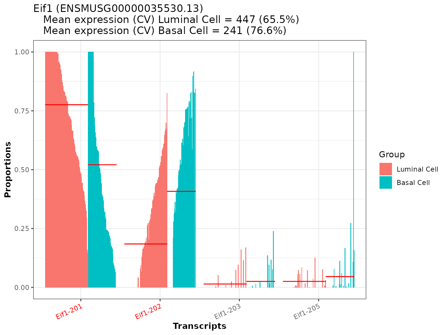
We see, that there are striking proportional differences for two of the transcripts of Eif1. There seems to be a significant shift in the expression proportions of Eif1-201 and Eif1-202 (as the names are marked in red). From the top annotation we can also see, that the mean total expression of Eif1 is higher in the Luminal Cell group - while the expression in the Basel Cell group is lower and also varies slightly more (coefficient of variation (CV) is higher).
For the interactive HTML-table we would need to save the images to disk (in the to-be-created sub folder “images” of the current working directory). There is also a convenience option, to directly add the file paths to the dtu_table. As multiple plots are created, we can provide a BiocParallel object to speed up the creation. If no specific genes are provided, all significant genes will be plotted.
dturtle <- plot_proportion_barplot(dturtle = dturtle,
                                   meta_gene_id = "gene_id.1",
                                   savepath = "images",
                                   add_to_table = "barplot",
                                   BPPARAM = biocpar)
#> Creating 162 plots:
#>
  |
  |                                                                      |   0%
  |
  |=======                                                               |  10%
  |
  |==============                                                        |  20%
  |
  |=====================                                                 |  30%
  |
  |============================                                          |  40%
  |
  |===================================                                   |  50%
  |
  |==========================================                            |  60%
  |
  |=================================================                     |  70%
  |
  |========================================================              |  80%
  |
  |===============================================================       |  90%
  |
|======================================================================| 100%head(dturtle$dtu_table$barplot) #> [1] "images/Fstl1_barplot.png" "images/Lhfp_barplot.png" #> [3] "images/Hunk_barplot.png" "images/Hdgfl3_barplot.png" #> [5] "images/Spock2_barplot.png" "images/Rnf185_barplot.png" head(list.files("./images/")) #> [1] "Abhd14a_barplot.png" "Acpp_barplot.png" "Adk_barplot.png" #> [4] "Amd1_barplot.png" "Ank2_barplot.png" "Anxa7_barplot.png"
Proportion heatmap
A different visualization option is a heatmap, where additional meta data can be displayed alongside the transcript proportions (plot_proportion_pheatmap()). This visualization uses the pheatmap package, the user can specify any of the available parameters to customize the results.
temp <- plot_proportion_pheatmap(dturtle = dturtle, genes = "Eif1",
                                 sample_meta_table_columns = c("sample_id","condition"),
                                 include_expression = TRUE, treeheight_col=20)
#> Creating 1 plots:
temp$Eif1
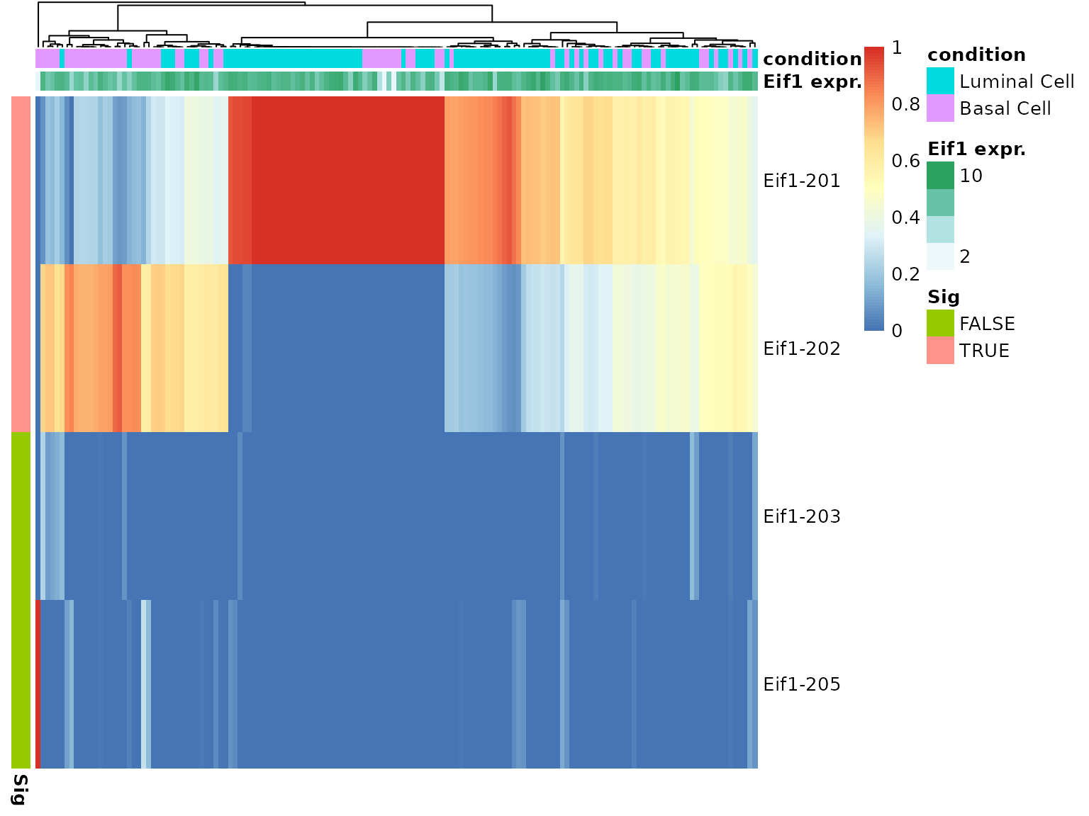
By default, row and column annotations are added. This plot helps to examine the transcript composition of groups of cells. We can see a block of samples solely expressing Eif1-201, majorly from the Luminal Cell group.
Again, we can save the plots to disk and add them to the dtu_table:
dturtle <- plot_proportion_pheatmap(dturtle = dturtle,
                                    include_expression = TRUE,
                                    treeheight_col=20,
                                    sample_meta_table_columns = c("sample_id","condition"),
                                    savepath = "images",
                                    add_to_table = "pheatmap",
                                    BPPARAM = biocpar)
#> Creating 162 plots:
#>
  |
  |                                                                      |   0%
  |
  |=======                                                               |  10%
  |
  |==============                                                        |  20%
  |
  |=====================                                                 |  30%
  |
  |============================                                          |  40%
  |
  |===================================                                   |  50%
  |
  |==========================================                            |  60%
  |
  |=================================================                     |  70%
  |
  |========================================================              |  80%
  |
  |===============================================================       |  90%
  |
|======================================================================| 100%head(dturtle$dtu_table$pheatmap) #> [1] "images/Fstl1_pheatmap.png" "images/Lhfp_pheatmap.png" #> [3] "images/Hunk_pheatmap.png" "images/Hdgfl3_pheatmap.png" #> [5] "images/Spock2_pheatmap.png" "images/Rnf185_pheatmap.png" head(list.files("./images/")) #> [1] "Abhd14a_barplot.png" "Abhd14a_pheatmap.png" "Acpp_barplot.png" #> [4] "Acpp_pheatmap.png" "Adk_barplot.png" "Adk_pheatmap.png"
Transcript overview
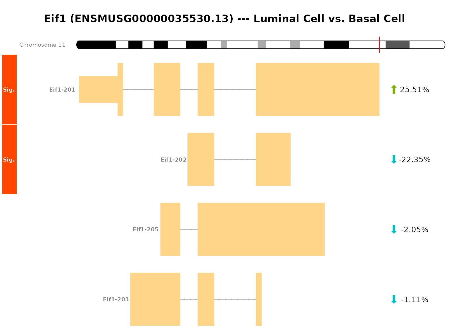
Until now, we looked at the different transcripts as abstract entities. Alongside proportional differences, the actual difference in the exon-intron structure of transcripts is of great importance for many research questions. This structure can be visualized with the plot_transcripts_view() functionality of DTUrtle.
This visualization is based on the Gviz package and needs a path to a GTF file (or a read-in object). In Import and format data we already imported a GTF file. This was subset to transcript-level (via the import_gtf() function), thus this is not sufficient for the visualization. We can reuse the actual GTF file though, which should in general match with the one used for the tx2gene data frame.
As we have ensured the one_to_one mapping in Import and format data and potentially renamed some genes, we should specify the one_to_one parameter in this call.
plot_transcripts_view(dturtle = dturtle,
                              genes = "Eif1",
                              gtf = "../gencode.vM24.annotation_spike.gtf",
                              genome = 'mm10',
                              one_to_one = TRUE)
#>
#> Importing gtf file from disk.
#>
#> Performing one to one mapping in gtf
#>
#> Found gtf GRanges for 1 of 1 provided genes.
#>
#> Fetching ideogram tracks ...
#> Creating 1 plots:
#> $Eif1
#> $Eif1$chr11
#> Ideogram track 'chr11' for chromosome 11 of the mm10 genome
#>
#> $Eif1$OverlayTrack
#> OverlayTrack 'OverlayTrack' containing 2 subtracks
#>
#> $Eif1$OverlayTrack
#> OverlayTrack 'OverlayTrack' containing 2 subtracks
#>
#> $Eif1$OverlayTrack
#> OverlayTrack 'OverlayTrack' containing 2 subtracks
#>
#> $Eif1$OverlayTrack
#> OverlayTrack 'OverlayTrack' containing 2 subtracks
#>
#> $Eif1$titles
#> An object of class "ImageMap"
#> Slot "coords":
#>              x1       y1   x2        y2
#> chr11         6 120.0000 58.2  186.8141
#> OverlayTrack  6 186.8141 58.2  426.6106
#> OverlayTrack  6 426.6106 58.2  666.4070
#> OverlayTrack  6 666.4070 58.2  906.2035
#> OverlayTrack  6 906.2035 58.2 1146.0000
#>
#> Slot "tags":
#> $title
#>          chr11   OverlayTrack   OverlayTrack   OverlayTrack   OverlayTrack
#>        "chr11" "OverlayTrack" "OverlayTrack" "OverlayTrack" "OverlayTrack"
This visualization shows the structure of the transcripts of Eif1. Our significant transcripts (Eif1-201 and Eif1-202) are quite different to each other. Eif1-201 has a different first exon than Eif1-202, which first exon is partially consisting of a conserved intron sequence. The arrows on the right side indicate the mean fitted proportional change in the comparison groups, thus showing a over-expression of Eif1-201 in Luminal Cell compared to Basal Cell.
The areas between exons indicate intron sequences, which have been compressed in this representation to highlight the exon structure. Only consensus introns are compressed to a defined minimal size. This can be turned off with reduce_introns=FALSE or alternatively reduced introns can be highlighted by setting a colorful reduce_introns_fill.
Analogous as before, we can save plots to disk and add them to the dtu_table:
dturtle <- plot_transcripts_view(dturtle = dturtle,
                                 gtf = "../gencode.vM24.annotation_spike.gtf",
                                 genome = 'mm10',
                                 one_to_one = TRUE,
                                 savepath = "images",
                                 add_to_table = "transcript_view",
                                 BPPARAM = biocpar)
#>
#> Importing gtf file from disk.
#>
#> Performing one to one mapping in gtf
#>
#> Found gtf GRanges for 162 of 162 provided genes.
#>
#> Fetching ideogram tracks ...
#> Creating 162 plots:
#>
  |
  |                                                                      |   0%
  |
  |=======                                                               |  10%
  |
  |==============                                                        |  20%
  |
  |=====================                                                 |  30%
  |
  |============================                                          |  40%
  |
  |===================================                                   |  50%
  |
  |==========================================                            |  60%
  |
  |=================================================                     |  70%
  |
  |========================================================              |  80%
  |
  |===============================================================       |  90%
  |
|======================================================================| 100%head(dturtle$dtu_table$transcript_view) #> [1] "images/Fstl1_transcripts.png" "images/Lhfp_transcripts.png" #> [3] "images/Hunk_transcripts.png" "images/Hdgfl3_transcripts.png" #> [5] "images/Spock2_transcripts.png" "images/Rnf185_transcripts.png" head(list.files("./images/")) #> [1] "Abhd14a_barplot.png" "Abhd14a_pheatmap.png" #> [3] "Abhd14a_transcripts.png" "Acpp_barplot.png" #> [5] "Acpp_pheatmap.png" "Acpp_transcripts.png"
Visualize DTU table
The dturtle$dtu_table is now ready to be visualized as an interactive HTML-table. Please note, that it is optional to add any plots or additional columns to the table. Thus the visualization will work directly after calling create_dtu_table().
The dtu_table object looks like this:
head(dturtle$dtu_table)
#>        gene_ID  gene_qvalue minimal_tx_qvalue number_tx number_significant_tx
#> Fstl1    Fstl1 1.566420e-29      7.933080e-33         4                     3
#> Lhfp      Lhfp 1.224028e-09      1.551439e-12         4                     2
#> Hunk      Hunk 7.663673e-03      9.168634e-04         3                     2
#> Hdgfl3  Hdgfl3 6.025880e-06      0.000000e+00         2                     2
#> Spock2  Spock2 4.619053e-06      0.000000e+00         2                     2
#> Rnf185  Rnf185 5.014701e-05      0.000000e+00         2                     2
#>        max(Luminal Cell-Basal Cell) chromosome tx_expr_in_max
#> Fstl1                     0.8464848      chr16      0.4133333
#> Lhfp                      0.8116508       chr3      0.2266667
#> Hunk                      0.7807970      chr16      0.1266667
#> Hdgfl3                   -0.7640278       chr7      0.1466667
#> Spock2                   -0.7582541      chr10      0.2066667
#> Rnf185                    0.7465166      chr11      0.1933333
#>                          barplot                   pheatmap
#> Fstl1   images/Fstl1_barplot.png  images/Fstl1_pheatmap.png
#> Lhfp     images/Lhfp_barplot.png   images/Lhfp_pheatmap.png
#> Hunk     images/Hunk_barplot.png   images/Hunk_pheatmap.png
#> Hdgfl3 images/Hdgfl3_barplot.png images/Hdgfl3_pheatmap.png
#> Spock2 images/Spock2_barplot.png images/Spock2_pheatmap.png
#> Rnf185 images/Rnf185_barplot.png images/Rnf185_pheatmap.png
#>                      transcript_view
#> Fstl1   images/Fstl1_transcripts.png
#> Lhfp     images/Lhfp_transcripts.png
#> Hunk     images/Hunk_transcripts.png
#> Hdgfl3 images/Hdgfl3_transcripts.png
#> Spock2 images/Spock2_transcripts.png
#> Rnf185 images/Rnf185_transcripts.png
Before creating the actual table, we can optionally define column formatter functions, which color the specified columns. The coloring might help with to quickly dissect the results.
DTUrtle come with some pre-defined column formatter functions (for p-values and percentages), other formatter functions from the formattable package can also be used. Advanced users might also define their own functions.
We create a named list, linking column names to formatter functions:
column_formatter_list <- list(
      "gene_qvalue" = table_pval_tile("white", "orange", digits = 3),
      "minimal_tx_qvalue" = table_pval_tile("white", "orange", digits = 3),
      "number_tx" = formattable::color_tile('white', "lightblue"),
      "number_significant_tx" = formattable::color_tile('white', "lightblue"),
      "max(Luminal Cell-Basal Cell)" = table_percentage_bar('lightgreen', "#FF9999", digits=2),
      "tx_expr_in_max" = table_percentage_bar('white', "lightblue", color_break = 0, digits=2))
This column_formatter_list is subsequently provided to plot_dtu_table():
plot_dtu_table(dturtle = dturtle, savepath = "my_results.html",
               column_formatters = column_formatter_list)
Note: ️As seen above, the paths to the plots are relative. Please make sure that the saving directory in
plot_dtu_table()is correctly set and the plots are reachable from that directory with the given path.The links in the following example are just for demonstration purposes and do not work!
For later use we can save the final DTUrtle object to disk:
saveRDS(dturtle, "./dturtle_res.RDS")
Comparison to Tabula Muris single-cell data
The data set used in the Tabula Muris vignette, and this data set are of the same tissue from the same species (mammary gland tissue of mouse). So it is of interest to inspect how big the overlap between called DTU and DGE genes between data sets are, obviously if the same cell types are compared. Notably, we do not expect a complete overlap, as differing sequencing protocols were used, a 10X chromium protocol with high cell-numbers but a rather shallow sequencing depth in the Tabula Muris data set, and the Smart-seq2 protocol with a high sequencing depth, but rather low cell numbers. Furthermore, differing mouse strains and even more importantly, differing developmental stages were analyzed - thus affecting the comparability. Nonetheless, we would common key marker genes to pop up in the analysis of both data sets.
As the analysis presented in the Tabula Muris vignette focuses on cell types, which are not present in both data sets, we have to quickly re-run the DTU and DGE analysis with common cell types. For this we choose the comparison of luminal cells versus basal cells. For simplicity, we import the counts and meta data table generated in the Tabula Muris vignette (representing the data state before performing the DTU analysis - thus after the last step of the Sample metadata part).
Comparison of DTU results
We simply redo the DTU analysis, just with different cell types that shall be compared:
dtu_tab_mur <- run_drimseq(counts = tab_mur_cts, tx2gene = tx2gene, pd=tab_mur_pd,
                    cond_col = "cell_ontology_class", cond_levels = c("luminal epithelial cell of mammary gland", "basal cell"), filtering_strategy = "sc",
                    BPPARAM = biocpar)
#> Using tx2gene columns:
#>  transcript_name ---> 'feature_id'
#>  gene_name ---> 'gene_id'
#>
#> Comparing in 'cell_ontology_class': 'luminal epithelial cell of mammary gland' vs 'basal cell'
#> Excluding 3630 cells/samples for this comparison!
#>
#> Proceed with cells/samples:
#> luminal epithelial cell of mammary gland
#>                                      459
#>                               basal cell
#>                                      392
#>
#> Filtering...
#>
  |
  |                                                                      |   0%
  |
  |=======                                                               |  10%
  |
  |==============                                                        |  20%
  |
  |=====================                                                 |  30%
  |
  |============================                                          |  40%
  |
  |===================================                                   |  50%
  |
  |==========================================                            |  60%
  |
  |=================================================                     |  70%
  |
  |========================================================              |  80%
  |
  |===============================================================       |  90%
  |
  |======================================================================| 100%
#> Retain 30236 of 74243 features.
#> Removed 44007 features.
#>
#> Performing statistical tests...
#> * Calculating mean gene expression..
#> * Estimating common precision..
#> ! Using common_precision = 21.2862 as prec_init !
#> * Estimating genewise precision..
#> ! Using loess fit as a shrinkage factor !
#> * Fitting the DM model..
#>    Using the one way approach.
#> * Fitting the BB model..
#>    Using the one way approach.
#> * Fitting the DM model..
#>    Using the one way approach.
#> * Calculating likelihood ratio statistics..
#> * Fitting the BB model..
#>    Using the one way approach.
#> * Calculating likelihood ratio statistics..
dtu_tab_mur <- posthoc_and_stager(dturtle = dtu_tab_mur, ofdr = 0.05, posthoc = 0.1)
#> Posthoc filtered 20513 features.
#> The returned adjusted p-values are based on a stage-wise testing approach and are only valid for the provided target OFDR level of 5%. If a different target OFDR level is of interest,the entire adjustment should be re-run.
#> Found 835 significant genes with 1310 significant transcripts (OFDR: 0.05)
Now we can simply calculate the amount of overlapping significant DTU genes:
common_dtu_genes <- intersect(dturtle$sig_gene, dtu_tab_mur$sig_gene)
length(common_dtu_genes)
#> [1] 55
Lastly, we can compute the fraction of overlapping elements compared to the length of the smaller set (so that we can achieve an actual overlap of 100%):
Comparison of DGE results
We can do the same for the DGE analysis. As the tabula muris data did not underwent scaling for the DTU analysis, we can simply summarize the transcript-level counts to gene-level for DGE calling. Please note, that this only works in this special case (no scaling during import because of a 3’-biased UMI-based protocol) - if that is not the case please re-import the data via import_dge_counts().
tab_mur_dge_cts <- summarize_to_gene(tab_mur_cts, tx2gene = tx2gene)
dge_tab_mur <- run_deseq2(counts = tab_mur_dge_cts, pd=tab_mur_pd, cond_col = "cell_ontology_class",
                          cond_levels = c("luminal epithelial cell of mammary gland", "basal cell"),
                          dge_calling_strategy = "sc", lfc_threshold = 1, sig_threshold = 0.01, BPPARAM = biocpar)
#>
#> Comparing in 'cell_ontology_class': 'luminal epithelial cell of mammary gland' vs 'basal cell'
#> Excluding 3630 cells/samples for this comparison!
#>
#> Proceed with cells/samples:
#> luminal epithelial cell of mammary gland
#>                                      459
#>                               basal cell
#>                                      392
#> converting counts to integer mode
#>   Note: levels of factors in the design contain characters other than
#>   letters, numbers, '_' and '.'. It is recommended (but not required) to use
#>   only letters, numbers, and delimiters '_' or '.', as these are safe characters
#>   for column names in R. [This is a message, not a warning or an error]
#> Warning in (function (object, test = c("Wald", "LRT"), fitType =
#> c("parametric", : parallelization of DESeq() is not implemented for
#> fitType='glmGamPoi'
#> estimating size factors
#> estimating dispersions
#> gene-wise dispersion estimates: 10 workers
#> mean-dispersion relationship
#> final dispersion estimates, fitting model and testing: 10 workers
#> using 'apeglm' for LFC shrinkage. If used in published research, please cite:
#>     Zhu, A., Ibrahim, J.G., Love, M.I. (2018) Heavy-tailed prior distributions for
#>     sequence count data: removing the noise and preserving large differences.
#>     Bioinformatics. https://doi.org/10.1093/bioinformatics/bty895
#> computing FSOS 'false sign or small' s-values (T=1)
#> Found 3178 significant DEGs.
#>      Over-expressed: 2465
#>      Under-expressed: 713
Again, we can calculate the amount of overlapping significant DGE genes and the overlap fraction compared to the size of the smaller set:
common_dge_genes <- intersect(dturtle$dge_analysis$results_sig$gene, dge_tab_mur$results_sig$gene)
length(common_dge_genes)
#> [1] 852
length(common_dge_genes)/min(length(dturtle$dge_analysis$results_sig$gene), length(dge_tab_mur$results_sig$gene))
#> [1] 0.442138
We see the overlap fraction for the DTU analysis results (~34%) is slightly lower than the overlap fraction of the DGE analysis results (~44%). This is somewhat expected, if we consider the problem size to solve in the individual analyses. It is very reassuring though, that the same luminal cell marker-transcript genes are again identified in the DTU analysis as before in the Tabular Muris vignette:
Session info
Computation time for this vignette:
#> Time difference of 1.97361 hours#> R version 3.6.2 (2019-12-12)
#> Platform: x86_64-pc-linux-gnu (64-bit)
#> Running under: Debian GNU/Linux 10 (buster)
#>
#> Matrix products: default
#> BLAS/LAPACK: /usr/lib/x86_64-linux-gnu/libopenblasp-r0.3.5.so
#>
#> locale:
#> [1] LC_CTYPE=en_US.UTF-8 LC_NUMERIC=C
#> [3] LC_TIME=en_US.UTF-8 LC_COLLATE=en_US.UTF-8
#> [5] LC_MONETARY=en_US.UTF-8 LC_MESSAGES=C
#> [7] LC_PAPER=en_US.UTF-8 LC_NAME=C
#> [9] LC_ADDRESS=C LC_TELEPHONE=C
#> [11] LC_MEASUREMENT=en_US.UTF-8 LC_IDENTIFICATION=C
#>
#> attached base packages:
#> [1] stats graphics grDevices utils datasets methods base
#>
#> other attached packages:
#> [1] DTUrtle_1.0.2 sparseDRIMSeq_0.1.2
#>
#> loaded via a namespace (and not attached):
#> [1] backports_1.1.10 Hmisc_4.4-1
#> [3] BiocFileCache_1.10.2 systemfonts_0.3.2
#> [5] plyr_1.8.6 lazyeval_0.2.2
#> [7] splines_3.6.2 crosstalk_1.1.0.1
#> [9] BiocParallel_1.22.0 GenomeInfoDb_1.22.1
#> [11] ggplot2_3.3.2 digest_0.6.26
#> [13] ensembldb_2.10.2 stageR_1.10.0
#> [15] htmltools_0.5.0 formattable_0.2.0.1
#> [17] magrittr_2.0.1 checkmate_2.0.0
#> [19] memoise_1.1.0 BSgenome_1.54.0
#> [21] cluster_2.1.0 limma_3.42.2
#> [23] Biostrings_2.54.0 readr_1.4.0
#> [25] annotate_1.64.0 matrixStats_0.57.0
#> [27] askpass_1.1 bdsmatrix_1.3-4
#> [29] pkgdown_1.6.1 prettyunits_1.1.1
#> [31] jpeg_0.1-8.1 colorspace_1.4-1
#> [33] blob_1.2.1 rappdirs_0.3.1
#> [35] apeglm_1.8.0 textshaping_0.1.2
#> [37] xfun_0.18 dplyr_1.0.2
#> [39] crayon_1.3.4 RCurl_1.98-1.2
#> [41] jsonlite_1.7.1 tximport_1.16.1
#> [43] genefilter_1.68.0 VariantAnnotation_1.32.0
#> [45] survival_3.1-8 glue_1.4.2
#> [47] gtable_0.3.0 zlibbioc_1.32.0
#> [49] XVector_0.26.0 DelayedArray_0.12.3
#> [51] BiocGenerics_0.32.0 scales_1.1.1
#> [53] pheatmap_1.0.12 mvtnorm_1.1-1
#> [55] DBI_1.1.0 edgeR_3.28.1
#> [57] Rcpp_1.0.5 xtable_1.8-4
#> [59] progress_1.2.2 emdbook_1.3.12
#> [61] htmlTable_2.1.0 foreign_0.8-72
#> [63] bit_4.0.4 Formula_1.2-4
#> [65] DT_0.16 stats4_3.6.2
#> [67] htmlwidgets_1.5.2 httr_1.4.2
#> [69] RColorBrewer_1.1-2 ellipsis_0.3.1
#> [71] pkgconfig_2.0.3 XML_3.99-0.3
#> [73] farver_2.0.3 Gviz_1.30.4
#> [75] nnet_7.3-12 dbplyr_1.4.4
#> [77] locfit_1.5-9.4 tidyselect_1.1.0
#> [79] labeling_0.4.2 rlang_0.4.11
#> [81] reshape2_1.4.4 AnnotationDbi_1.48.0
#> [83] munsell_0.5.0 tools_3.6.2
#> [85] generics_0.0.2 RSQLite_2.2.1
#> [87] evaluate_0.14 stringr_1.4.0
#> [89] yaml_2.2.1 ragg_0.4.0
#> [91] knitr_1.30 bit64_4.0.5
#> [93] fs_1.5.0 purrr_0.3.4
#> [95] AnnotationFilter_1.10.0 mime_0.9
#> [97] grr_0.9.5 biomaRt_2.42.1
#> [99] compiler_3.6.2 rstudioapi_0.11
#> [101] curl_4.3 png_0.1-7
#> [103] tibble_3.0.4 geneplotter_1.64.0
#> [105] glmGamPoi_1.5.0 stringi_1.5.3
#> [107] GenomicFeatures_1.38.2 desc_1.2.0
#> [109] lattice_0.20-38 ProtGenerics_1.18.0
#> [111] Matrix_1.2-18 vctrs_0.3.4
#> [113] pillar_1.4.6 lifecycle_1.0.1
#> [115] data.table_1.13.2 bitops_1.0-6
#> [117] Matrix.utils_0.9.8 rtracklayer_1.46.0
#> [119] GenomicRanges_1.38.0 R6_2.4.1
#> [121] latticeExtra_0.6-29 gridExtra_2.3
#> [123] IRanges_2.20.2 dichromat_2.0-0
#> [125] MASS_7.3-51.4 assertthat_0.2.1
#> [127] SummarizedExperiment_1.16.1 openssl_1.4.3
#> [129] DESeq2_1.33.1 rprojroot_1.3-2
#> [131] GenomicAlignments_1.22.1 Rsamtools_2.2.3
#> [133] S4Vectors_0.24.4 GenomeInfoDbData_1.2.2
#> [135] parallel_3.6.2 hms_0.5.3
#> [137] grid_3.6.2 rpart_4.1-15
#> [139] coda_0.19-4 rmarkdown_2.5
#> [141] biovizBase_1.34.1 bbmle_1.0.23.1
#> [143] numDeriv_2016.8-1.1 Biobase_2.46.0
#> [145] base64enc_0.1-3