Analysis of Tabular Muris mouse single-cell RNA-seq data
Tobias Tekath
2021-11-18
Source:vignettes/Tabular_Muris_mouse_single-cell_analysis.Rmd
Tabular_Muris_mouse_single-cell_analysis.RmdThis vignette exemplifies the analysis of single-cell RNA-seq data with DTUrtle. The data used in this vignette is publicly available as Bioproject PRJNA432002 and the used FASTQ-files can be downloaded from here. The corresponding publication can be found here.
The following code shows an example of an DTUrtle workflow. Assume we have performed the pre-processing as described here and the R working directory is a newly created folder called dtu_results.
Setup
Load the DTUrtle package and set the BiocParallel parameter. It is recommended to perform computations in parallel, if possible.
library(DTUrtle)
#> Loading required package: sparseDRIMSeq
#> To cite DTUrtle in publications use:
#>
#>  Tobias Tekath, Martin Dugas.
#>  Differential transcript usage analysis
#>  of bulk and single-cell RNA-seq data with DTUrtle.
#>  Bioinformatics,
#>  2021.
#>  https://doi.org/10.1093/bioinformatics/btab629.
#>
#> Use citation(DTUrtle) for BibTeX information.
#use up to 10 cores for computation
biocpar <- BiocParallel::MulticoreParam(10)
Import and format data
We want to start by reading in our quantification counts, as well as a file specifying which transcript ID or name belongs to which gene ID or name.
Importing and processing GTF annotation (tx2gene)
To get this transcript to gene (tx2gene) mapping, we will utilize the already present Gencode annotation file gencode.vM24.annotation.gtf. The import_gtf() function utilizes the a rtracklayer package and returns a transcript-level filtered version of the available data.
tx2gene <- import_gtf(gtf_file = "../gencode.vM24.annotation.gtf")
head(tx2gene, n=3)
#>   seqnames   start     end width strand  source       type score phase
#> 1     chr1 3073253 3074322  1070      +  HAVANA transcript    NA    NA
#> 2     chr1 3102016 3102125   110      + ENSEMBL transcript    NA    NA
#> 3     chr1 3205901 3216344 10444      -  HAVANA transcript    NA    NA
#>                gene_id        transcript_id      gene_type     gene_name
#> 1 ENSMUSG00000102693.1 ENSMUST00000193812.1            TEC 4933401J01Rik
#> 2 ENSMUSG00000064842.1 ENSMUST00000082908.1          snRNA       Gm26206
#> 3 ENSMUSG00000051951.5 ENSMUST00000162897.1 protein_coding          Xkr4
#>        transcript_type   transcript_name level transcript_support_level
#> 1                  TEC 4933401J01Rik-201     2                       NA
#> 2                snRNA       Gm26206-201     3                       NA
#> 3 processed_transcript          Xkr4-203     2                        1
#>        mgi_id   tag          havana_gene    havana_transcript protein_id ccdsid
#> 1 MGI:1918292 basic OTTMUSG00000049935.1 OTTMUST00000127109.1       <NA>   <NA>
#> 2 MGI:5455983 basic                 <NA>                 <NA>       <NA>   <NA>
#> 3 MGI:3528744  <NA> OTTMUSG00000026353.2 OTTMUST00000086625.1       <NA>   <NA>
#>    ont
#> 1 <NA>
#> 2 <NA>
#> 3 <NA>
There are a lot of columns present in the data frame, but at the moment we are mainly interested in the columns gene_id, gene_name, transcript_id and transcript_name.
As we want to use gene and transcript names as the main identifiers in our analysis (so we can directly say: Gene x is differential), we should ensure that each gene / transcript name maps only to a single gene / transcript id.
For this we can use the DTUrtle function one_to_one_mapping(), which checks if there are identifiers, which relate to the same name. If this is the case, the names (not the identifiers) are slightly altered by appending a number. If id_x and id_y both have the name ABC, the id_y name is altered to ABC_2 by default.
tx2gene$gene_name <- one_to_one_mapping(name = tx2gene$gene_name, id = tx2gene$gene_id)
#> Changed 109 names.
tx2gene$transcript_name <- one_to_one_mapping(name = tx2gene$transcript_name, id = tx2gene$transcript_id)
#> No changes needed -> already one to one mapping.
We see that it was a good idea to ensure the one to one mapping, as many doublets have been corrected.
For the run_drimseq() tx2gene parameter, we need a data frame, where the first column specifies the transcript identifiers and the second column specifying the corresponding gene names. Rather than subsetting the data frame, a column reordering is proposed, so that additional data can still be used in further steps. DTUrtle makes sure to carry over additional data columns in the analysis steps. To reorder the columns of our tx2gene data frame, we can utilize the move_columns_to_front() functionality.
tx2gene <- move_columns_to_front(df = tx2gene, columns = c("transcript_name", "gene_name"))
head(tx2gene, n=5)
#>     transcript_name     gene_name seqnames   start     end  width strand
#> 1 4933401J01Rik-201 4933401J01Rik     chr1 3073253 3074322   1070      +
#> 2       Gm26206-201       Gm26206     chr1 3102016 3102125    110      +
#> 3          Xkr4-203          Xkr4     chr1 3205901 3216344  10444      -
#> 4          Xkr4-202          Xkr4     chr1 3206523 3215632   9110      -
#> 5          Xkr4-201          Xkr4     chr1 3214482 3671498 457017      -
#>    source       type score phase              gene_id        transcript_id
#> 1  HAVANA transcript    NA    NA ENSMUSG00000102693.1 ENSMUST00000193812.1
#> 2 ENSEMBL transcript    NA    NA ENSMUSG00000064842.1 ENSMUST00000082908.1
#> 3  HAVANA transcript    NA    NA ENSMUSG00000051951.5 ENSMUST00000162897.1
#> 4  HAVANA transcript    NA    NA ENSMUSG00000051951.5 ENSMUST00000159265.1
#> 5  HAVANA transcript    NA    NA ENSMUSG00000051951.5 ENSMUST00000070533.4
#>        gene_type      transcript_type level transcript_support_level
#> 1            TEC                  TEC     2                       NA
#> 2          snRNA                snRNA     3                       NA
#> 3 protein_coding processed_transcript     2                        1
#> 4 protein_coding processed_transcript     2                        1
#> 5 protein_coding       protein_coding     2                        1
#>        mgi_id   tag          havana_gene    havana_transcript
#> 1 MGI:1918292 basic OTTMUSG00000049935.1 OTTMUST00000127109.1
#> 2 MGI:5455983 basic                 <NA>                 <NA>
#> 3 MGI:3528744  <NA> OTTMUSG00000026353.2 OTTMUST00000086625.1
#> 4 MGI:3528744  <NA> OTTMUSG00000026353.2 OTTMUST00000086624.1
#> 5 MGI:3528744  CCDS OTTMUSG00000026353.2 OTTMUST00000065166.1
#>             protein_id      ccdsid  ont
#> 1                 <NA>        <NA> <NA>
#> 2                 <NA>        <NA> <NA>
#> 3                 <NA>        <NA> <NA>
#> 4                 <NA>        <NA> <NA>
#> 5 ENSMUSP00000070648.4 CCDS14803.1 <NA>
This concludes the tx2gene formatting.
Reading in quantification data
The read-in of the quantification counts can be achieved with import_counts(), which uses the tximport package in the background. This function is able to parse the output of many different quantification tools. Advanced users might be able to tune parameters to parse arbitrary output files from currently not supported tools.
In the pre-processing vignette we quantified the counts with Alevin. The folder structure of the quantification results folder looks like this:
list.files("../alevin/")
#> [1] "10X_P7_12" "10X_P7_13" "index"     "txmap.tsv"
We will create a named files vector, pointing to the quants_mat.gz file for each sample. The names help to differentiate the samples later on.
files <- Sys.glob("../alevin/10X_P7_*/alevin/quants_mat.gz")
names(files) <- basename(gsub("/alevin/quants_mat.gz", "", files))
The files object looks like this:
#>                                  10X_P7_12
#> "../alevin/10X_P7_12/alevin/quants_mat.gz"
#>                                  10X_P7_13
#> "../alevin/10X_P7_13/alevin/quants_mat.gz"
The actual import will be performed with import_counts().
cts_list <- import_counts(files = files, type = "alevin")
#> Reading in 2 alevin runs.
#> importing alevin data is much faster after installing `fishpond` (>= 1.2.0)
#> reading in alevin gene-level counts across cells
#> importing alevin data is much faster after installing `fishpond` (>= 1.2.0)
#> reading in alevin gene-level counts across cells
The cts_list object is a named list, with a sparse Matrix per sample. In single-cell data, each sample normally consists of many different cells with an unique cell barcode. These cell barcodes might overlap between samples though. For this reason, many single-cell workflow use a cell barcode extension, uniquely assigning each cell to a sample. This can also be done in DTUrtle with combine_to_matrix(), which is only applicable if you are analyzing single-cell data.
This function will make sure that there are no duplicated barcodes between you samples, before merging the matrices together. If there are duplicated barcodes, a cell extension is added. Additionally, all not expressed features are removed to reduce the size of the data.
To have matching cell names with the sample annotation we add in the next step, we set the cell extensions explicitly and prepend them.
cts <- combine_to_matrix(tx_list = cts_list, cell_extensions = c("10X_P7_12", "10X_P7_13"), cell_extension_side = "prepend")
#> Found overall duplicated cellnames. Trying cellname extension per sample.
#> Map extensions:
#>  10X_P7_12 --> '10X_P7_12_'
#>  10X_P7_13 --> '10X_P7_13_'
#>
#> Merging matrices
#> Excluding 49494 overall not expressed features.
#> 91454 features left.
Apparently there were some duplicated cell barcodes between our samples, so a cell barcode extensions are useful either way.
dim(cts)
#> [1] 91454  8318
There are ~91k features left for 8318 cells.
Sample metadata
Finally, we need a sample metadata data frame, specifying which sample belongs to which comparison group. This table is also convenient to store and carry over additional metadata.
For single-cell data, this is not a sample metadata data frame, but a cell metadata data frame. We have to specify the information on cell level, with the barcodes as identifiers.
As we want to use the cell type assignments from the Tabula Muris project, we download the Robj file containing the annotation. The Tabula Muris Data has been deposited at Figshare
We can perform the download with the following bash code:
The meta.data data frame of this object contains the wanted annotation.
library(Seurat)
load("../droplet_Mammary_Gland_seurat_tiss.Robj", verbose=TRUE)
#> Loading objects:
#>   tiss

tabula_muris_metadata <- tiss@meta.data
dim(tabula_muris_metadata)
#> [1] 4481   15
head(tabula_muris_metadata, n=5)
#>                            nGene nUMI orig.ident   channel        tissue
#> 10X_P7_12_AAACCTGAGTTGAGAT  2125 7442        10X 10X_P7_12 Mammary_Gland
#> 10X_P7_12_AAACCTGTCGTCACGG  2750 9544        10X 10X_P7_12 Mammary_Gland
#> 10X_P7_12_AAACCTGTCTTGTACT  1837 6479        10X 10X_P7_12 Mammary_Gland
#> 10X_P7_12_AAACCTGTCTTTAGTC  2051 7284        10X 10X_P7_12 Mammary_Gland
#> 10X_P7_12_AAACGGGCAGTGGGAT  1129 3797        10X 10X_P7_12 Mammary_Gland
#>                            subtissue mouse.sex mouse.id percent.ercc
#> 10X_P7_12_AAACCTGAGTTGAGAT                   F   3-F-56            0
#> 10X_P7_12_AAACCTGTCGTCACGG                   F   3-F-56            0
#> 10X_P7_12_AAACCTGTCTTGTACT                   F   3-F-56            0
#> 10X_P7_12_AAACCTGTCTTTAGTC                   F   3-F-56            0
#> 10X_P7_12_AAACGGGCAGTGGGAT                   F   3-F-56            0
#>                            percent.ribo         free_annotation
#> 10X_P7_12_AAACCTGAGTTGAGAT    0.2758667 luminal progenitor cell
#> 10X_P7_12_AAACCTGTCGTCACGG    0.2768231                    <NA>
#> 10X_P7_12_AAACCTGTCTTGTACT    0.1967896                    <NA>
#> 10X_P7_12_AAACCTGTCTTTAGTC    0.2397035                    <NA>
#> 10X_P7_12_AAACGGGCAGTGGGAT    0.4234922                    <NA>
#>                                                 cell_ontology_class res.1
#> 10X_P7_12_AAACCTGAGTTGAGAT luminal epithelial cell of mammary gland     6
#> 10X_P7_12_AAACCTGTCGTCACGG                                   B cell     1
#> 10X_P7_12_AAACCTGTCTTGTACT                             stromal cell     3
#> 10X_P7_12_AAACCTGTCTTTAGTC                             stromal cell     3
#> 10X_P7_12_AAACGGGCAGTGGGAT                                   B cell     1
#>                            cluster.ids cell_ontology_id
#> 10X_P7_12_AAACCTGAGTTGAGAT           6       CL:0002326
#> 10X_P7_12_AAACCTGTCGTCACGG           1       CL:0000236
#> 10X_P7_12_AAACCTGTCTTGTACT           3       CL:0000499
#> 10X_P7_12_AAACCTGTCTTTAGTC           3       CL:0000499
#> 10X_P7_12_AAACGGGCAGTGGGAT           1       CL:0000236
As we have only cell type information available for cells analyzed in Tabula Muris, we subset our data set to the matching cells.
All 4481 cells from Tabula Muris have been recovered. The tabula_muris_metadata data frame can be used as our meta data table.
For an example workflow utilizing the Seurat object directly, please see Workflow with Seurat object
(optional) Estimate influence of priming-bias
As the 10X Chromium 3’ protocol preferentially generates reads of the 3’-end of an mRNA, DTU effects of some specific transcripts might not be detectable. DTUrtle offers a novel scoring scheme, called “detection probability”, to assess which transcripts might be prone to be impaired by such a bias. This score can be computed with the DTUrtle function priming_bias_detection_probability().
The score calculation can be summarized like this: For each gene, a reference transcript is chosen (based on the expression data, selecting the major proportionally expressed transcript as reference). Each other transcript of a gene is now compared to this reference transcript, calculating where the first detectable exon-level difference occurs between the transcript entities - and at what relative coordinate this difference is located (looking from the priming enriched end). Based on this information, a detection probability is calculated, with 1 indicating no influence of the prime-biased reads on the detection ability and 0 indicating a very heavy influence. Thus, DTU effects for transcripts with a low score would be expected less likely to be detectable with the given data.
We can add this score information to an already existing table, like the tx2gene table (add_to_table = tx2gene). As we need exon-level information for the calculation, we should provide an unfiltered GTF GRanges or data frame object - or alternatively a file path.
unfilt_gtf <- import_gtf("../gencode.vM24.annotation.gtf", feature_type = NULL, out_df = FALSE)
#set priming_enrichment to '3', as we expect reads enriched towards the 3' end of the mRNA.
tx2gene <- priming_bias_detection_probability(counts = cts, tx2gene = tx2gene, gtf = unfilt_gtf, one_to_one = TRUE,
                                              priming_enrichment = "3", add_to_table = tx2gene, BPPARAM = biocpar)
#>
#> Performing one to one mapping in gtf
#>
#> Found gtf GRanges for 55385 of 55385 provided genes.
#> Scoring transcripts of 55385 genes.
#>
  |
  |                                                                      |   0%
  |
  |=======                                                               |  10%
  |
  |==============                                                        |  20%
  |
  |=====================                                                 |  30%
  |
  |============================                                          |  40%
  |
  |===================================                                   |  50%
  |
  |==========================================                            |  60%
  |
  |=================================================                     |  70%
  |
  |========================================================              |  80%
  |
  |===============================================================       |  90%
  |
  |======================================================================| 100%
The newly added columns are detection_probability and used_as_ref:
head(tx2gene[,c("transcript_name", "gene_name", "detection_probability", "used_as_ref")])
#>     transcript_name     gene_name detection_probability used_as_ref
#> 1 4933401J01Rik-201 4933401J01Rik             1.0000000       FALSE
#> 2       Gm26206-201       Gm26206             1.0000000       FALSE
#> 3          Xkr4-203          Xkr4             1.0000000        TRUE
#> 4          Xkr4-202          Xkr4             0.7340248       FALSE
#> 5          Xkr4-201          Xkr4             0.4870666       FALSE
#> 6       Gm18956-201       Gm18956             1.0000000       FALSE
We can calculate, that a potential 3’-bias would not influence the majority of annotated transcripts, relevant for the DTU analysis:
#only genes with at least two transcript isoforms are relevant for DTU analysis
dtu_relevant_genes <- unique(tx2gene$gene_name[duplicated(tx2gene$gene_name)])
summary(tx2gene$detection_probability[tx2gene$gene_name %in% dtu_relevant_genes])
#>     Min.  1st Qu.   Median     Mean  3rd Qu.     Max.
#> 0.000138 0.394984 1.000000 0.719740 1.000000 1.000000
DTU analysis
We have prepared all necessary data to perform the differentially transcript usage (DTU) analysis. DTUrtle only needs two simple commands to perform it. Please be aware that these steps are the most compute intensive and, depending on your data, might take some time to complete. It is recommended to parallelize the computations with the BBPARAM parameter, if applicable.
First, we want to set-up and perform the statistical analysis with DRIMSeq, a DTU specialized statistical framework utilizing a Dirichlet-multinomial model. This can be done with the run_drimseq() command. We use the previously imported data as parameters, specifying which column in the cell metadata data frame contains ids and which the group information we want. We should also specify which of the groups should be compared (if there are more than two) and in which order. The order given in the cond_levels parameter also specifies the comparison formula.
In this example we choose two specific cell types (from the column cell_ontology_class) and do not specify the id column, as rownames are chosen by default.
Note: By default
run_drimseq()converts sparse count matrix to a dense format for statistical computations (force_dense=TRUE). While this increases memory usage, it currently also reduces the run time. The computations can be performed keeping the sparse counts by settingforce_dense=FALSE.
dturtle <- run_drimseq(counts = cts, tx2gene = tx2gene, pd=tabula_muris_metadata,
                    cond_col = "cell_ontology_class",
                    cond_levels = c("T cell", "luminal epithelial cell of mammary gland"),
                    filtering_strategy = "sc", BPPARAM = biocpar)
#> Using tx2gene columns:
#>  transcript_name ---> 'feature_id'
#>  gene_name ---> 'gene_id'
#>
#> Comparing in 'cell_ontology_class': 'T cell' vs 'luminal epithelial cell of mammary gland'
#> Excluding 2272 cells/samples for this comparison!
#>
#> Proceed with cells/samples:
#>                                   T cell
#>                                     1750
#> luminal epithelial cell of mammary gland
#>                                      459
#>
#> Filtering...
#>
  |
  |                                                                      |   0%
  |
  |=======                                                               |  10%
  |
  |==============                                                        |  20%
  |
  |=====================                                                 |  30%
  |
  |============================                                          |  40%
  |
  |===================================                                   |  50%
  |
  |==========================================                            |  60%
  |
  |=================================================                     |  70%
  |
  |========================================================              |  80%
  |
  |===============================================================       |  90%
  |
  |======================================================================| 100%
#> Retain 32578 of 78489 features.
#> Removed 45911 features.
#>
#> Performing statistical tests...
#> * Calculating mean gene expression..
#> * Estimating common precision..
#> ! Using common_precision = 21.2862 as prec_init !
#> * Estimating genewise precision..
#> ! Using loess fit as a shrinkage factor !
#> * Fitting the DM model..
#>    Using the one way approach.
#> * Fitting the BB model..
#>    Using the one way approach.
#> * Fitting the DM model..
#>    Using the one way approach.
#> * Calculating likelihood ratio statistics..
#> * Fitting the BB model..
#>    Using the one way approach.
#> * Calculating likelihood ratio statistics..
As in all statistical procedures, it is of favor to perform as few tests as possible but as much tests as necessary, to maintain a high statistical power. This is achieved by filtering the data to remove inherently uninteresting items, for example very lowly expressed genes or features. DTUrtle includes a powerful and customizable filtering functionality for this task, which is an optimized version of the dmFilter() function of the DRIMSeq package.
Above we used a predefined filtering strategy for single-cell data, requiring that features contribute at least 5% of the total expression in at least 5% of the cells of the smallest group. Additionally, all genes are filtered, which only have a single transcript left, as they can not be analyzed in DTU analysis. The filtering options can be extended or altered by the user.
dturtle$used_filtering_options
#> $DRIM
#> $DRIM$min_samps_gene_expr
#> [1] 0
#>
#> $DRIM$min_samps_feature_expr
#> [1] 0
#>
#> $DRIM$min_samps_feature_prop
#> [1] 22.95
#>
#> $DRIM$min_gene_expr
#> [1] 0
#>
#> $DRIM$min_feature_expr
#> [1] 0
#>
#> $DRIM$min_feature_prop
#> [1] 0.05
#>
#> $DRIM$run_gene_twice
#> [1] TRUE
The resulting dturtle object will be used as our main results object, storing all necessary and interesting data of the analysis. It is a simple and easy-accessible list, which can be easily extended / altered by the user. By default three different meta data tables are generated:
-
meta_table_gene: Contains gene level meta data. -
meta_table_tx: Contains transcript level meta data. -
meta_table_sample: Contains sample level meta data (as the createdpddata frame)
These meta data tables are used in for visualization purposes and can be extended by the user.
head(dturtle$meta_table_gene, n=5)
#>                        gene     exp_in exp_in_T cell
#> 0610009B22Rik 0610009B22Rik 0.07424174   0.024571429
#> 0610010F05Rik 0610010F05Rik 0.02580353   0.007428571
#> 0610010K14Rik 0610010K14Rik 0.28700770   0.222285714
#> 0610030E20Rik 0610030E20Rik 0.16115890   0.120571429
#> 1110004F10Rik 1110004F10Rik 0.43549117   0.368571429
#>               exp_in_luminal epithelial cell of mammary gland seqnames strand
#> 0610009B22Rik                                      0.26361656    chr11      -
#> 0610010F05Rik                                      0.09586057    chr11      -
#> 0610010K14Rik                                      0.53376906    chr11      -
#> 0610030E20Rik                                      0.31590414     chr6      +
#> 1110004F10Rik                                      0.69063181     chr7      +
#>                     type             gene_id.1      gene_type
#> 0610009B22Rik transcript  ENSMUSG00000007777.9 protein_coding
#> 0610010F05Rik transcript ENSMUSG00000042208.15 protein_coding
#> 0610010K14Rik transcript ENSMUSG00000020831.18 protein_coding
#> 0610030E20Rik transcript  ENSMUSG00000058706.5 protein_coding
#> 1110004F10Rik transcript ENSMUSG00000030663.12 protein_coding
This table shows the single genes, together with their total expressed-in ratio (“exp_in”), the specific expressed-in ratios in the specific comparison groups, as well with other information from the provided GTF-file.
As proposed in Love et al. (2018), we will use a two-stage statistical testing procedure together with a post-hoc filtering on the standard deviations in proportions (posthoc_and_stager()). We will use stageR to determine genes, that show a overall significant change in transcript proportions. For these significant genes, we will try to pinpoint specific transcripts, which significantly drive this overall change. As a result, we will have a list of significant genes (genes showing the overall change) and a list of significant transcripts (one or more transcripts of the significant genes). Please note, that not every significant gene does have one or more significant transcripts. It is not always possible to attribute the overall change in proportions to single transcripts. These two list of significant items are computed and corrected against a overall false discovery rate (OFDR).
Additionally, we will apply a post-hoc filtering scheme to improve the targeted OFDR control level. The filtering strategy will discard transcripts, which standard deviation of the proportion per cell/sample is below the specified threshold. For example by setting posthoc=0.1, we will exclude all transcripts, which proportional expression (in regard to the total gene expression) deviates by less than 0.1 between cells. This filtering step should mostly exclude ‘uninteresting’ transcripts, which would not have been called as significant either way.
dturtle <- posthoc_and_stager(dturtle = dturtle, ofdr = 0.05, posthoc = 0.1)
#> Posthoc filtered 25829 features.
#> The returned adjusted p-values are based on a stage-wise testing approach and are only valid for the provided target OFDR level of 5%. If a different target OFDR level is of interest,the entire adjustment should be re-run.
#> Found 2100 significant genes with 3130 significant transcripts (OFDR: 0.05)
The dturtle object now contains additional elements, including the lists of significant genes and significant transcripts.
head(dturtle$sig_gene)
#> [1] "1110004F10Rik" "1110008P14Rik" "1110032A03Rik" "1110038B12Rik"
#> [5] "1700037C18Rik" "1810058I24Rik"
head(dturtle$sig_tx)
#>       1110008P14Rik       1110008P14Rik       1110032A03Rik       1110032A03Rik
#> "1110008P14Rik-202" "1110008P14Rik-201" "1110032A03Rik-201" "1110032A03Rik-206"
#>       1110038B12Rik       2310009A05Rik
#> "1110038B12Rik-201" "2310009A05Rik-201"
(optional) DGE analysis
Alongside a DTU analysis, a DGE analysis might be of interest for your research question. DTUrtle offers a basic DGE calling workflow for bulk and single-cell RNA-seq data via DESeq2.
To utilize this workflow, we should re-scale our imported counts. The transcript-level count matrix has been scaled for the DTU analysis, but for a DGE analysis un-normalized counts should be used (as DESeq2 normalizes internally). We can simply re-import the count data, by providing the already defined files object to the DGE analysis specific function import_dge_counts(). This function will make sure that the counts are imported but not scaled and also summarizes to gene-level.
Our files object looks like this:
head(files)
#>                                  10X_P7_12
#> "../alevin/10X_P7_12/alevin/quants_mat.gz"
#>                                  10X_P7_13
#> "../alevin/10X_P7_13/alevin/quants_mat.gz"
We re-import the files and use combine_to_matrix() to create one big matrix (as we did for the DTU analysis):
cts_dge <- import_dge_counts(files, type="alevin", tx2gene=tx2gene)
#> Reading in 2 alevin runs.
#> importing alevin data is much faster after installing `fishpond` (>= 1.2.0)
#> reading in alevin gene-level counts across cells
#> importing alevin data is much faster after installing `fishpond` (>= 1.2.0)
#> reading in alevin gene-level counts across cells
cts_dge <- combine_to_matrix(tx_list = cts_dge, cell_extensions = c("10X_P7_12", "10X_P7_13"), cell_extension_side = "prepend")
#> Found overall duplicated cellnames. Trying cellname extension per sample.
#> Map extensions:
#>  10X_P7_12 --> '10X_P7_12_'
#>  10X_P7_13 --> '10X_P7_13_'
#>
#> Merging matrices
#> Excluding 25835 overall not expressed features.
#> 28496 features left.
With this data, we can perform the DGE analysis with DESeq2 with the DTUrtle function run_deseq2(). DESeq2 is one of the gold-standard tools for DGE calling in bulk RNA-seq data and showed very good performance for single-cell data in multiple benchmarks. The DESeq2 vignette recommends adjusting some parameters for DGE analysis of single-cell data - DTUrtle incorporates these recommendations and adjusts the specific parameters based on the provided dge_calling_strategy.
After the DESeq2 DGE analysis, the estimated log2 fold changes are shrunken (preferably with apeglm) - to provide a secondary ranking variable beside the statistical significance. If a shrinkage with apeglm is performed, run_deseq2() defaults to also compute s-values rather than adjusted p-values. The underlying hypothesis for s-values and (standard) p-values differs slightly, with s-values hypothesis being presumably preferential in a real biological context. Far more information about all these topics can be found in the excellent DESeq2 vignette and the associated publications.
run_deseq2() will tell the user, if one or more advised packages are missing. It is strongly advised to follow these recommendations.
dturtle$dge_analysis <- run_deseq2(counts = cts_dge, pd = tabula_muris_metadata, cond_col = "cell_ontology_class",
                                   cond_levels = c("T cell", "luminal epithelial cell of mammary gland"), lfc_threshold = 1,
                                   sig_threshold = 0.01, dge_calling_strategy = "sc", BPPARAM = biocpar)
#>
#> Comparing in 'cell_ontology_class': 'T cell' vs 'luminal epithelial cell of mammary gland'
#> Excluding 2272 cells/samples for this comparison!
#>
#> Proceed with cells/samples:
#>                                   T cell
#>                                     1750
#> luminal epithelial cell of mammary gland
#>                                      459
#> converting counts to integer mode
#>   Note: levels of factors in the design contain characters other than
#>   letters, numbers, '_' and '.'. It is recommended (but not required) to use
#>   only letters, numbers, and delimiters '_' or '.', as these are safe characters
#>   for column names in R. [This is a message, not a warning or an error]
#> Warning in (function (object, test = c("Wald", "LRT"), fitType =
#> c("parametric", : parallelization of DESeq() is not implemented for
#> fitType='glmGamPoi'
#> estimating size factors
#> estimating dispersions
#> gene-wise dispersion estimates: 10 workers
#> mean-dispersion relationship
#> final dispersion estimates, fitting model and testing: 10 workers
#> using 'apeglm' for LFC shrinkage. If used in published research, please cite:
#>     Zhu, A., Ibrahim, J.G., Love, M.I. (2018) Heavy-tailed prior distributions for
#>     sequence count data: removing the noise and preserving large differences.
#>     Bioinformatics. https://doi.org/10.1093/bioinformatics/bty895
#> computing FSOS 'false sign or small' s-values (T=1)
#> Found 11071 significant DEGs.
#>      Over-expressed: 552
#>      Under-expressed: 10519
We provided a log2 fold change threshold of 1 (on log2 scale), thus preferring an effect size of 2x or more. The output of run_deseq2() is a list, containing various elements (see run_deseq2()’s description). This result list can easily added to an existing DTUrtle object, as shown above.
We can now identify genes which show both a DGE and DTU signal:
dtu_dge_genes <- intersect(dturtle$sig_gene, dturtle$dge_analysis$results_sig$gene)
length(dtu_dge_genes)
#> [1] 1717
Result aggregation and visualization
The DTUrtle package contains multiple visualization options, enabling an in-depth inspection.
DTU table creation
We will start by aggregating the analysis results to a data frame with create_dtu_table(). This function is highly flexible and allows aggregation of gene or transcript level metadata in various ways. By default some useful information are included in the dtu table, in this example we further specify to include the seqnames column of the gene level metadata (which contains chromosome information) as well as the maximal expressed in ratio per cell type from the transcript level metadata (“expressed in” specifies the ratio of cells, were the expression of the gene / transcript is > 0). Furthermore we add the a column with the absolute difference between the expressed in ratios.
dturtle <- create_dtu_table(dturtle = dturtle, add_gene_metadata = list("chromosome"="seqnames"),
                               add_tx_metadata = list("max_tx_expr_in_T_cell" = c("exp_in_T cell", max),
                                                      "max_tx_expr_in_luminal_epithelial_cell_of_mammary_gland" =
                                                        c("exp_in_luminal epithelial cell of mammary gland", max)))

# add absolute difference between "expressed in" columns.
dturtle$dtu_table$abs_diff_expr_in <- abs(dturtle$dtu_table$max_tx_expr_in_T_cell-dturtle$dtu_table$max_tx_expr_in_luminal_epithelial_cell_of_mammary_gland)
head(dturtle$dtu_table, n=5)
#>           gene_ID   gene_qvalue minimal_tx_qvalue number_tx
#> Pde4d       Pde4d 2.507274e-209     1.631713e-169         5
#> Atp6v0e2 Atp6v0e2  2.576117e-21      3.358998e-23         3
#> Lamb3       Lamb3  2.737907e-65      3.706752e-66         4
#> Cgref1     Cgref1  1.990326e-36      0.000000e+00         2
#> Nr6a1       Nr6a1  2.403643e-37      2.382682e-40         4
#>          number_significant_tx
#> Pde4d                        3
#> Atp6v0e2                     1
#> Lamb3                        1
#> Cgref1                       2
#> Nr6a1                        1
#>          max(T cell-luminal epithelial cell of mammary gland) chromosome
#> Pde4d                                              -0.8201809      chr13
#> Atp6v0e2                                            0.8084999       chr6
#> Lamb3                                               0.7969231       chr1
#> Cgref1                                             -0.7603835       chr5
#> Nr6a1                                               0.7230380       chr2
#>          max_tx_expr_in_T_cell
#> Pde4d               0.16514286
#> Atp6v0e2            0.03028571
#> Lamb3               0.16400000
#> Cgref1              0.05257143
#> Nr6a1               0.08742857
#>          max_tx_expr_in_luminal_epithelial_cell_of_mammary_gland
#> Pde4d                                                  0.5098039
#> Atp6v0e2                                               0.1938998
#> Lamb3                                                  0.1677560
#> Cgref1                                                 0.3246187
#> Nr6a1                                                  0.1633987
#>          abs_diff_expr_in
#> Pde4d         0.344661064
#> Atp6v0e2      0.163614068
#> Lamb3         0.003755991
#> Cgref1        0.272047308
#> Nr6a1         0.075970121
This table is our basis for creating an interactive HTML-table of the results.
The column definitions are as follows:
- “gene_ID”: Gene name or identifier used for the analysis.
- “gene_qvalue”: Multiple testing corrected p-value (a.k.a. q-value) comparing all transcripts together between the two groups (“gene level”).
- “minimal_tx_qvalue”: The minimal multiple testing corrected p-value from comparing all transcripts individually between the two groups (“transcript level”). I.e. the q-value of the most significant transcript.
- “number_tx”: The number of analyzed transcripts for the specific gene.
- “number_significant_tx”: The number of significant transcripts from the ‘transcript level’ analysis.
- “max(T cell-luminal epithelial cell of mammary gland)”: Maximal proportional difference between the two groups (T cell vs luminal epithelial cell of mammary gland). E.g. one transcript of ‘Pde4d’ is ~82% more expressed in ‘luminal epithelial cell of mammary gland’ cells compared to ‘T cell’ cells.
- “chromosome”: the chromosome the gene resides on.
Please note, that the columns and their meaning can easily be altered and redefined by the user.
Proportion barplot
As a first visualization option we will create a barplot of the proportions of each transcript per sample. We can use the function plot_proportion_barplot() for this task, which also adds the mean proportion fit per subgroup to the plot (by default as a red line).
As an example, we will create the plot for the gene Lcn2, which is one of the significant genes found in the analysis. We will optionally provide the gene_id for Lcn2, which is stored in the column gene_id.1 of dturtle$meta_table_gene.
temp <- plot_proportion_barplot(dturtle = dturtle, genes = "Lcn2", meta_gene_id = "gene_id.1")
#> Creating 1 plots:
temp$Lcn2
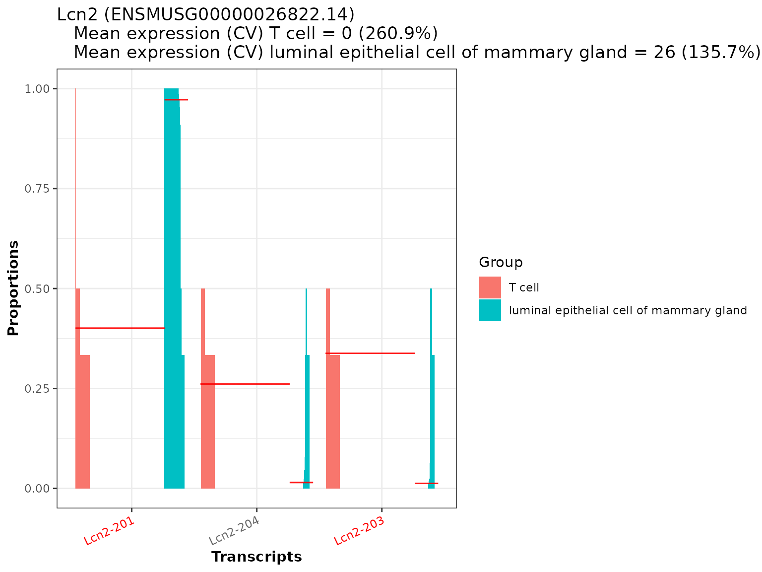
We see, that most of the proportional differences for Lcn2 are driven by 2 of the 3 transcripts (Lcn2-201 and Lcn2-203). These transcripts are also the significant transcripts found in the analysis (as they are marked in red). Notably 3 other transcripts of Lcn2 have been removed by the filtering thresholds in run_drimseq(). Lcn2-201 is proportionally overexpressed in luminal epithelial cell of mammary gland cells, in contrast to Lcn2-203 which is proportionally overexpressed in T cell cells. We additionally see, that the overall expression level of Lcn2 is way higher in luminal epithelial cell of mammary gland than in T cell.
For the interactive HTML-table we would need to save the images to disk (in the to-be-created sub folder “images” of the current working directory). There is also a convenience option, to directly add the file paths to the dtu_table. As multiple plots are created, we can provide a BiocParallel object to speed up the creation. If no specific genes are provided, all significant genes will be plotted.
dturtle <- plot_proportion_barplot(dturtle = dturtle,
                                   meta_gene_id = "gene_id.1",
                                   savepath = "images",
                                   add_to_table = "barplot",
                                   BPPARAM = biocpar)
#> Creating 2100 plots:
#>
  |
  |                                                                      |   0%
  |
  |=======                                                               |  10%
  |
  |==============                                                        |  20%
  |
  |=====================                                                 |  30%
  |
  |============================                                          |  40%
  |
  |===================================                                   |  50%
  |
  |==========================================                            |  60%
  |
  |=================================================                     |  70%
  |
  |========================================================              |  80%
  |
  |===============================================================       |  90%
  |
|======================================================================| 100%head(dturtle$dtu_table$barplot) #> [1] "images/Pde4d_barplot.png" "images/Atp6v0e2_barplot.png" #> [3] "images/Lamb3_barplot.png" "images/Cgref1_barplot.png" #> [5] "images/Nr6a1_barplot.png" "images/Rtn2_barplot.png" head(list.files("./images/")) #> [1] "Abca3_barplot.png" "Abcb9_barplot.png" "Abce1_barplot.png" #> [4] "Abhd17a_barplot.png" "Abhd2_barplot.png" "Abhd8_barplot.png"
Proportion heatmap
A different visualization option is a heatmap, where additional meta data can be displayed alongside the transcript proportions (plot_proportion_pheatmap()). This visualization uses the pheatmap package, the user can specify any of the available parameters to customize the results.
temp <- plot_proportion_pheatmap(dturtle = dturtle, genes = "Lcn2",
                                 sample_meta_table_columns = c("sample_id","condition"),
                                 include_expression = TRUE, treeheight_col=20)
#> Creating 1 plots:
temp$Lcn2
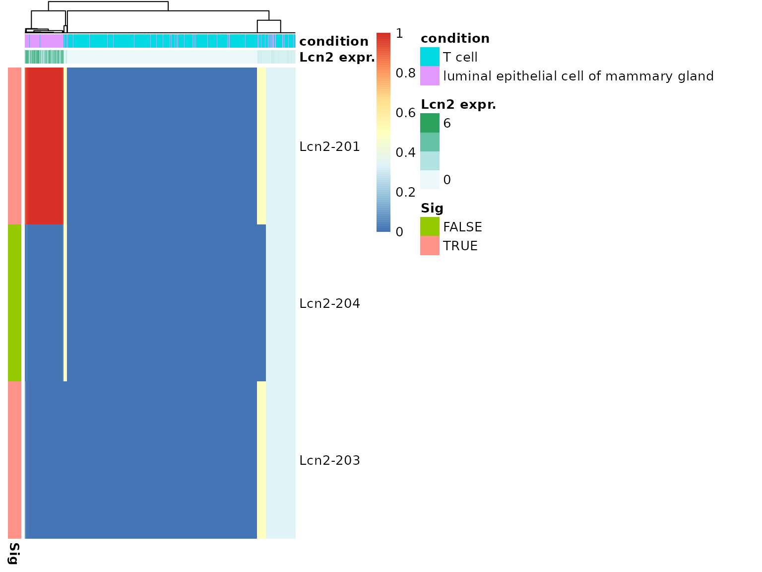
By default, row and column annotations are added. This plot helps to examine the transcript composition of groups of cells. We see, the vast majority of luminal epithelial cell of mammary gland cells are exclusively expressing Lcn2-201. The Lcn2 expressing cells of the T cell cells are mostly split-expressing Lcn2-201 and Lcn2-203. The significant transcripts are indicated by the row annotation on the left side of the heatmap.
Again, we can save the plots to disk and add them to the dtu_table:
dturtle <- plot_proportion_pheatmap(dturtle = dturtle,
                                    include_expression = TRUE,
                                    treeheight_col=20,
                                    sample_meta_table_columns = c("sample_id","condition"),
                                    savepath = "images",
                                    add_to_table = "pheatmap",
                                    BPPARAM = biocpar)
#> Creating 2100 plots:
#>
  |
  |                                                                      |   0%
  |
  |=======                                                               |  10%
  |
  |==============                                                        |  20%
  |
  |=====================                                                 |  30%
  |
  |============================                                          |  40%
  |
  |===================================                                   |  50%
  |
  |==========================================                            |  60%
  |
  |=================================================                     |  70%
  |
  |========================================================              |  80%
  |
  |===============================================================       |  90%
  |
|======================================================================| 100%head(dturtle$dtu_table$pheatmap) #> [1] "images/Pde4d_pheatmap.png" "images/Atp6v0e2_pheatmap.png" #> [3] "images/Lamb3_pheatmap.png" "images/Cgref1_pheatmap.png" #> [5] "images/Nr6a1_pheatmap.png" "images/Rtn2_pheatmap.png" head(list.files("./images/")) #> [1] "Abca3_barplot.png" "Abca3_pheatmap.png" "Abcb9_barplot.png" #> [4] "Abcb9_pheatmap.png" "Abce1_barplot.png" "Abce1_pheatmap.png"
Transcript overview
Until now, we looked at the different transcripts as abstract entities. Alongside proportional differences, the actual difference in the exon-intron structure of transcripts is of great importance for many research questions. This structure can be visualized with the plot_transcripts_view() functionality of DTUrtle.
This visualization is based on the Gviz package and needs a path to a GTF file (or a read-in object). In Import and format data we already imported a GTF file. This was subset to transcript-level (via the import_gtf() function), thus this is not sufficient for the visualization. We can reuse the actual GTF file though, which should in general match with the one used for the tx2gene data frame.
As we have ensured the one_to_one mapping in Import and format data and potentially renamed some genes, we should specify the one_to_one parameter in this call.
plot_transcripts_view(dturtle = dturtle,
                              genes = "Lcn2",
                              gtf = "../gencode.vM24.annotation.gtf",
                              genome = 'mm10',
                              one_to_one = TRUE)
#>
#> Importing gtf file from disk.
#>
#> Performing one to one mapping in gtf
#>
#> Found gtf GRanges for 1 of 1 provided genes.
#>
#> Fetching ideogram tracks ...
#> Creating 1 plots:

#> $Lcn2
#> $Lcn2$chr2
#> Ideogram track 'chr2' for chromosome 2 of the mm10 genome
#>
#> $Lcn2$OverlayTrack
#> OverlayTrack 'OverlayTrack' containing 2 subtracks
#>
#> $Lcn2$OverlayTrack
#> OverlayTrack 'OverlayTrack' containing 2 subtracks
#>
#> $Lcn2$OverlayTrack
#> OverlayTrack 'OverlayTrack' containing 2 subtracks
#>
#> $Lcn2$titles
#> An object of class "ImageMap"
#> Slot "coords":
#>              x1       y1   x2        y2
#> chr2          6 120.0000 58.2  186.8141
#> OverlayTrack  6 186.8141 58.2  506.5427
#> OverlayTrack  6 506.5427 58.2  826.2714
#> OverlayTrack  6 826.2714 58.2 1146.0000
#>
#> Slot "tags":
#> $title
#>           chr2   OverlayTrack   OverlayTrack   OverlayTrack
#>         "chr2" "OverlayTrack" "OverlayTrack" "OverlayTrack"
This visualization shows the structure of the transcripts of Lcn2. Our two significant transcripts (Lcn2-201 and Lcn2-203) are quite different, with alternative end points as well as some retained intron sequences in Lcn2-203. The arrows on the right side indicate the mean fitted proportional change in the comparison groups, thus showing a under-expression of Lcn2-201 in T cell compared to luminal epithelial cell of mammary gland.
The areas between exons indicate intron sequences, which have been compressed in this representation to highlight the exon structure. Only consensus introns are compressed to a defined minimal size. This can be turned off with reduce_introns=FALSE or alternatively reduced introns can be highlighted by setting a colorful reduce_introns_fill.
Analogous as before, we can save plots to disk and add them to the dtu_table:
dturtle <- plot_transcripts_view(dturtle = dturtle,
                                 gtf = "../gencode.vM24.annotation.gtf",
                                 genome = 'mm10',
                                 one_to_one = TRUE,
                                 savepath = "images",
                                 add_to_table = "transcript_view",
                                 BPPARAM = biocpar)
#>
#> Importing gtf file from disk.
#>
#> Performing one to one mapping in gtf
#>
#> Found gtf GRanges for 2100 of 2100 provided genes.
#>
#> Fetching ideogram tracks ...
#> Creating 2100 plots:
#>
  |
  |                                                                      |   0%
  |
  |=======                                                               |  10%
  |
  |==============                                                        |  20%
  |
  |=====================                                                 |  30%
  |
  |============================                                          |  40%
  |
  |===================================                                   |  50%
  |
  |==========================================                            |  60%
  |
  |=================================================                     |  70%
  |
  |========================================================              |  80%
  |
  |===============================================================       |  90%
  |
|======================================================================| 100%head(dturtle$dtu_table$transcript_view) #> [1] "images/Pde4d_transcripts.png" "images/Atp6v0e2_transcripts.png" #> [3] "images/Lamb3_transcripts.png" "images/Cgref1_transcripts.png" #> [5] "images/Nr6a1_transcripts.png" "images/Rtn2_transcripts.png" head(list.files("./images/")) #> [1] "Abca3_barplot.png" "Abca3_pheatmap.png" "Abca3_transcripts.png" #> [4] "Abcb9_barplot.png" "Abcb9_pheatmap.png" "Abcb9_transcripts.png"
Dimensional reduction
Most RNA-seq analysis perform some kind of dimensional reduction method to visualize the samples in two (or three) dimensions. This is most useful for single-cell data sets or bulk experiments with a very high number of samples.
For these kind of experiments, DTUrtle provides a functionality to visualize the proportional differences in dimensional reduction coordinates. For the visualization with plot_dimensional_reduction(), we need a data frame of two coordinates per cell / samples - presumably from a dimensional reduction method like PCA, TSNE or UMAP.
In this example data set, the tiss object (from Sample metadata) contains usable TSNE coordinates:
head(tiss@dr$tsne@cell.embeddings, n=5)
#>                               tSNE_1     tSNE_2
#> 10X_P7_12_AAACCTGAGTTGAGAT  15.82803 -25.601272
#> 10X_P7_12_AAACCTGTCGTCACGG  39.56226 -14.578341
#> 10X_P7_12_AAACCTGTCTTGTACT -26.24403  -5.222502
#> 10X_P7_12_AAACCTGTCTTTAGTC -29.54653   2.016900
#> 10X_P7_12_AAACGGGCAGTGGGAT  22.76953  -5.078945
We can provide this data frame directly to the reduction_df parameter of plot_dimensional_reduction() function:
temp <- plot_dimensional_reduction(dturtle = dturtle,
                           reduction_df = tiss@dr$tsne@cell.embeddings,
                           plot = "proportions", genes = "Lcn2", plot_scale = "free_y")
#> Retrieved coordinates for 2209 out of 2209 cells / samples.
#> Creating 1 plots:
grid::grid.draw(temp$Lcn2)
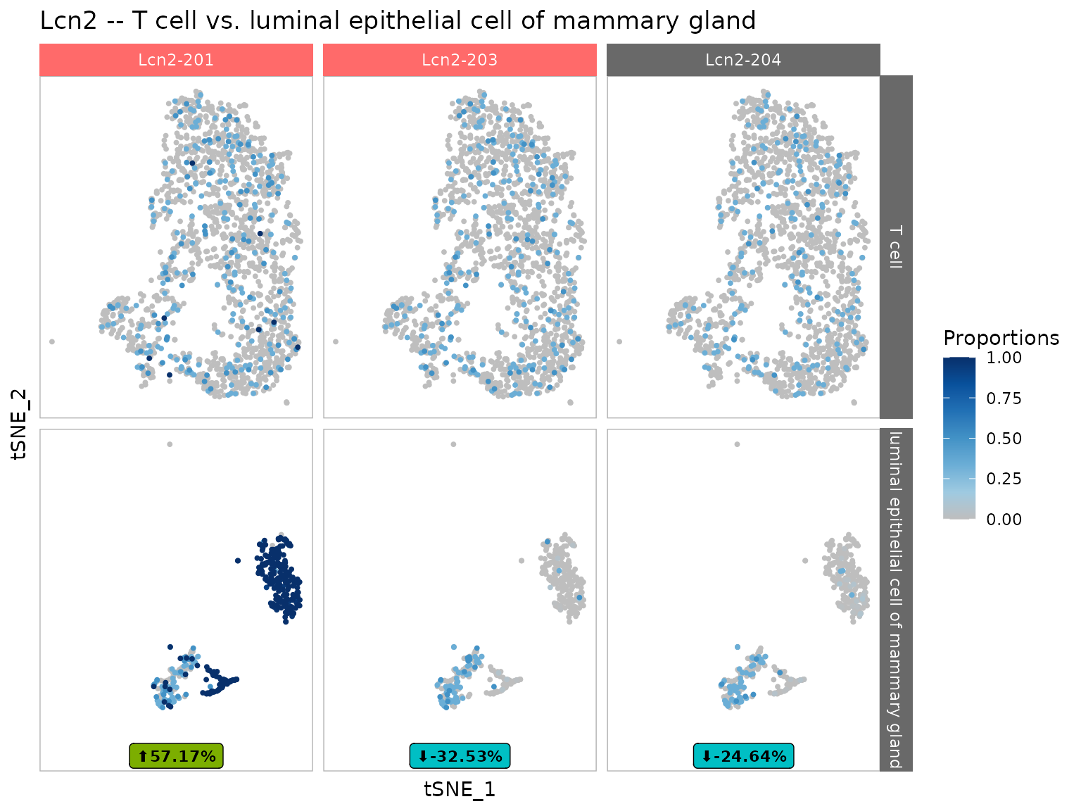
By default significant transcripts are highlighted by a red background name. Because of this modification, a grob object is returned. If indicate_significant_tx is set to FALSE, a more common ggplot2 object is returned.
Besides the actual transcript proportions, it is also possible to display the (log-transformed) expression values of the gene and the single transcripts in the plot.
dturtle <- plot_dimensional_reduction(dturtle = dturtle,
                                 reduction_df = tiss@dr$tsne@cell.embeddings,
                                 plot = "proportions",
                                 savepath = "images",
                                 add_to_table = "dimensional_reduction",
                                 BPPARAM = biocpar)
#> Retrieved coordinates for 2209 out of 2209 cells / samples.
#> Creating 2100 plots:
#>
  |
  |                                                                      |   0%
  |
  |=======                                                               |  10%
  |
  |==============                                                        |  20%
  |
  |=====================                                                 |  30%
  |
  |============================                                          |  40%
  |
  |===================================                                   |  50%
  |
  |==========================================                            |  60%
  |
  |=================================================                     |  70%
  |
  |========================================================              |  80%
  |
  |===============================================================       |  90%
  |
|======================================================================| 100%head(dturtle$dtu_table$transcript_view) #> [1] "images/Pde4d_transcripts.png" "images/Atp6v0e2_transcripts.png" #> [3] "images/Lamb3_transcripts.png" "images/Cgref1_transcripts.png" #> [5] "images/Nr6a1_transcripts.png" "images/Rtn2_transcripts.png" head(list.files("./images/")) #> [1] "Abca3_barplot.png" "Abca3_dim_reduce.png" "Abca3_pheatmap.png" #> [4] "Abca3_transcripts.png" "Abcb9_barplot.png" "Abcb9_dim_reduce.png"
Visualize DTU table
The dturtle$dtu_table is now ready to be visualized as an interactive HTML-table. Please note, that it is optional to add any plots or additional columns to the table. Thus the visualization will work directly after calling create_dtu_table().
The dtu_table object looks like this:
head(dturtle$dtu_table)
#>           gene_ID   gene_qvalue minimal_tx_qvalue number_tx
#> Pde4d       Pde4d 2.507274e-209     1.631713e-169         5
#> Atp6v0e2 Atp6v0e2  2.576117e-21      3.358998e-23         3
#> Lamb3       Lamb3  2.737907e-65      3.706752e-66         4
#> Cgref1     Cgref1  1.990326e-36      0.000000e+00         2
#> Nr6a1       Nr6a1  2.403643e-37      2.382682e-40         4
#> Rtn2         Rtn2  2.575898e-04      1.000000e+00         3
#>          number_significant_tx
#> Pde4d                        3
#> Atp6v0e2                     1
#> Lamb3                        1
#> Cgref1                       2
#> Nr6a1                        1
#> Rtn2                         0
#>          max(T cell-luminal epithelial cell of mammary gland) chromosome
#> Pde4d                                              -0.8201809      chr13
#> Atp6v0e2                                            0.8084999       chr6
#> Lamb3                                               0.7969231       chr1
#> Cgref1                                             -0.7603835       chr5
#> Nr6a1                                               0.7230380       chr2
#> Rtn2                                                0.7157688       chr7
#>          max_tx_expr_in_T_cell
#> Pde4d               0.16514286
#> Atp6v0e2            0.03028571
#> Lamb3               0.16400000
#> Cgref1              0.05257143
#> Nr6a1               0.08742857
#> Rtn2                0.01371429
#>          max_tx_expr_in_luminal_epithelial_cell_of_mammary_gland
#> Pde4d                                                 0.50980392
#> Atp6v0e2                                              0.19389978
#> Lamb3                                                 0.16775599
#> Cgref1                                                0.32461874
#> Nr6a1                                                 0.16339869
#> Rtn2                                                  0.06971678
#>          abs_diff_expr_in                     barplot
#> Pde4d         0.344661064    images/Pde4d_barplot.png
#> Atp6v0e2      0.163614068 images/Atp6v0e2_barplot.png
#> Lamb3         0.003755991    images/Lamb3_barplot.png
#> Cgref1        0.272047308   images/Cgref1_barplot.png
#> Nr6a1         0.075970121    images/Nr6a1_barplot.png
#> Rtn2          0.056002490     images/Rtn2_barplot.png
#>                              pheatmap                 transcript_view
#> Pde4d       images/Pde4d_pheatmap.png    images/Pde4d_transcripts.png
#> Atp6v0e2 images/Atp6v0e2_pheatmap.png images/Atp6v0e2_transcripts.png
#> Lamb3       images/Lamb3_pheatmap.png    images/Lamb3_transcripts.png
#> Cgref1     images/Cgref1_pheatmap.png   images/Cgref1_transcripts.png
#> Nr6a1       images/Nr6a1_pheatmap.png    images/Nr6a1_transcripts.png
#> Rtn2         images/Rtn2_pheatmap.png     images/Rtn2_transcripts.png
#>                   dimensional_reduction
#> Pde4d       images/Pde4d_dim_reduce.png
#> Atp6v0e2 images/Atp6v0e2_dim_reduce.png
#> Lamb3       images/Lamb3_dim_reduce.png
#> Cgref1     images/Cgref1_dim_reduce.png
#> Nr6a1       images/Nr6a1_dim_reduce.png
#> Rtn2         images/Rtn2_dim_reduce.png
Before creating the actual table, we can optionally define column formatter functions, which colour the specified columns. The colouring might help with to quickly dissect the results.
DTUrtle come with some pre-defined column formatter functions (for p-values and percentages), other formatter functions from the formattable package can also be used. Advanced users might also define their own functions.
We create a named list, linking column names to formatter functions:
column_formatter_list <- list(
      "gene_qvalue" = table_pval_tile("white", "orange", digits = 3),
      "minimal_tx_qvalue" = table_pval_tile("white", "orange", digits = 3),
      "number_tx" = formattable::color_tile('white', "lightblue"),
      "number_significant_tx" = formattable::color_tile('white', "lightblue"),
      "max(T cell-luminal epithelial cell of mammary gland)" = table_percentage_bar('lightgreen', "#FF9999", digits=2),
      "max_tx_expr_in_T_cell" = table_percentage_bar('white', "lightblue", color_break = 0, digits=2),
      "max_tx_expr_in_luminal_epithelial_cell_of_mammary_gland" = table_percentage_bar('white', "lightblue", color_break = 0, digits=2),
      "abs_diff_expr_in" = table_percentage_bar('white', "lightblue", color_break = 0, digits=2))
This column_formatter_list is subsequently provided to plot_dtu_table():
plot_dtu_table(dturtle = dturtle, savepath = "my_results.html",
               column_formatters = column_formatter_list)
Note: ️As seen above, the paths to the plots are relative. Please make sure that the saving directory in
plot_dtu_table()is correctly set and the plots are reachable from that directory with the given path.The links in the following example are just for demonstration purposes and do not work!
Workflow with Seurat object
As an Seurat object of the data set is already present in the Tabula muris publication, we can directly use this object in some DTUrtle analysis. Additionally, we can create an Seurat object containing both, gene and transcript level quantification data.
Seurat object and data import
We assume, you have followed this vignette till the Sample metadata section. The tiss Seurat object is still present from
load("../droplet_Mammary_Gland_seurat_tiss.Robj", verbose=TRUE)
#> Loading objects:
#>   tiss
tiss
#> An old seurat object
#>  23341 genes across 4481 samples
tiss@version
#> [1] '2.2.1'
We see the tiss object is a Seurat v2 object - DTUrtle can only process Seurat v3 or higher objects.
Luckily, there is a Seurat function to convert a v2 object to the v3 style:
tiss <- Seurat::UpdateSeuratObject(tiss)
#> Updating from v2.X to v3.X
#> Validating object structure
#> Updating object slots
#> Ensuring keys are in the proper strucutre
#> Ensuring feature names don't have underscores or pipes
#> Object representation is consistent with the most current Seurat version
tiss
#> An object of class Seurat
#> 23341 features across 4481 samples within 1 assay
#> Active assay: RNA (23341 features, 2432 variable features)
#>  2 dimensional reductions calculated: pca, tsne
tiss@version
#> [1] '3.2.2'
This updated object can now be used as input for the DTUrtle function combine_to_matrix(). We assume, we still have the cts_list object present from the initial import.
lapply(cts_list, dim)
#> $`10X_P7_12`
#> [1] 140948   3992
#>
#> $`10X_P7_13`
#> [1] 140948   4326
As in the workflow without the Seurat object, we want to combine the two matrices and subset the matrix to cells where we have metadata for (i.e. the cells present in the Seurat object).
We can achieve both tasks by directly supplying the Seurat object to the combine_to_matrix():
tiss <- combine_to_matrix(tx_list = cts_list, seurat_obj = tiss, tx2gene = tx2gene, cell_extension_side = "prepend")
#> Found overall duplicated cellnames. Trying cellname extension per sample.
#> Trying to infer cell extensions from Seurat object
#> Map extensions:
#>  10X_P7_12 --> '10X_P7_12_'
#>  10X_P7_13 --> '10X_P7_13_'
#>
#> Merging matrices
#> Of 8318 cells, 4481 (54%) could be found in the provided seurat object.
#> 3837 (46%) are unique to the transcriptomic files.
#> The seurat object contains 0 additional cells.
#> Subsetting!
#> Excluding 51930 overall not expressed features.
#> 89018 features left.
#> Adding assay 'dtutx'
We supply the list of count matrices per sample (cts_list), as well as the Seurat object. When a Seurat object is present, DTUrtle tries to infer the used cellname extensions from the Seurat object - which works in this case as expected and we do not have to provide the cell extensions by our own. Optionally, we can also provide the tx2gene when supplying a Seurat object, than the transcript to gene mapping will be added to the metadata of the newly created Seurat Assay.
tiss
#> An object of class Seurat
#> 112359 features across 4481 samples within 2 assays
#> Active assay: dtutx (89018 features, 0 variable features)
#>  1 other assay present: RNA
#>  2 dimensional reductions calculated: pca, tsne
tiss@active.assay
#> [1] "dtutx"
We see, the active assay of the Seurat object changed (to ‘dtutx’) and that assay contains way more features than before (as these are transcript level counts).
Adding the a transcript level assay to the Seurat object is quite handy for downstream functionality. The tiss object can now be handled as any other Seurat object, but returns transcript-level results by default.
This Seurat object can be used in the downstream DTUrtle pipeline instead of the cts object, alternatively we can pull the actual count matrix from the object:
seur_cts <- Seurat::GetAssayData(tiss)
dim(seur_cts)
#> [1] 89018  4481
dim(cts)
#> [1] 91454  4481
We can see a subtle difference in the number of features here. This is due to the fact, that the original cts was created taking all original 8318 cells into account (and filtering all not expressed features) - while the seur_cts object was subset to the 4481 we want to use before excluding not expressed features.
This difference has no downstream effect, as not expressed features are also excluded in the run_drimseq() filtering step.
As a sanity check, we can see if these two matrices are identical (at least for common features):
Identify cell type specific transcripts
As an example for downstream use of a Seurat object with transcript level information, we can use established Seurat functions to identify cell type specific transcripts. These cell types are annotated in the Seurat object:
table(tiss$cell_ontology_class)
#>
#>                                   B cell
#>                                      743
#>                               basal cell
#>                                      392
#>                         endothelial cell
#>                                      251
#> luminal epithelial cell of mammary gland
#>                                      459
#>                               macrophage
#>                                      186
#>                             stromal cell
#>                                      700
#>                                   T cell
#>                                     1750
We can identify cell type specific transcripts via Seurats FindAllMarkers functionality. Please note, that this marker identification is based on transcript counts, not proportions - thus it does not render a DTU analysis obsolete. It offers a quick way to identify transcripts, which are almost solely expressed in a single cell type.
#set cell types as active ident
Idents(tiss) <- tiss$cell_ontology_class
tiss <- NormalizeData(tiss)
cell_markers <- FindAllMarkers(tiss, only.pos=TRUE)
#> Calculating cluster luminal epithelial cell of mammary gland
#> Calculating cluster B cell
#> Calculating cluster stromal cell
#> Calculating cluster T cell
#> Calculating cluster endothelial cell
#> Calculating cluster basal cell
#> Calculating cluster macrophage
Apparently, we identified quite a lot of transcript as markers:
dim(cell_markers)
#> [1] 5776    7

head(cell_markers, n = 5)
#>            p_val avg_logFC pct.1 pct.2 p_val_adj
#> Krt18-201      0  3.281501 1.000 0.307         0
#> Wfdc18-201     0  3.229780 0.736 0.093         0
#> Krt19-201      0  3.087161 0.996 0.250         0
#> Krt8-201       0  2.838430 1.000 0.304         0
#> Epcam-204      0  2.543355 1.000 0.239         0
#>                                             cluster       gene
#> Krt18-201  luminal epithelial cell of mammary gland  Krt18-201
#> Wfdc18-201 luminal epithelial cell of mammary gland Wfdc18-201
#> Krt19-201  luminal epithelial cell of mammary gland  Krt19-201
#> Krt8-201   luminal epithelial cell of mammary gland   Krt8-201
#> Epcam-204  luminal epithelial cell of mammary gland  Epcam-204
We can split the markers by their cell type:
table(cell_markers$cluster)
#>
#> luminal epithelial cell of mammary gland
#>                                      761
#>                                   B cell
#>                                      471
#>                             stromal cell
#>                                      965
#>                                   T cell
#>                                      494
#>                         endothelial cell
#>                                     1381
#>                               basal cell
#>                                     1207
#>                               macrophage
#>                                      497
We can search for marker transcripts, which were also identified in the DTU analysis (between T cell and luminal epithelial cell of mammary gland):
#select common transcripts
dtu_markers <- cell_markers[cell_markers$gene %in% dturtle$sig_tx,]
table(dtu_markers$cluster)
#>
#> luminal epithelial cell of mammary gland
#>                                      274
#>                                   B cell
#>                                       97
#>                             stromal cell
#>                                      145
#>                                   T cell
#>                                      161
#>                         endothelial cell
#>                                      262
#>                               basal cell
#>                                      326
#>                               macrophage
#>                                       77
We see many markers, which have also been identified in the DTU analysis, are for the expected cell types (luminal epithelial cell of mammary gland and T cell). This becomes even more prominent, when we take the total amount of markers per cell type into account:
table(dtu_markers$cluster)/table(cell_markers$cluster)
#>
#> luminal epithelial cell of mammary gland
#>                                0.3600526
#>                                   B cell
#>                                0.2059448
#>                             stromal cell
#>                                0.1502591
#>                                   T cell
#>                                0.3259109
#>                         endothelial cell
#>                                0.1897176
#>                               basal cell
#>                                0.2700911
#>                               macrophage
#>                                0.1549296
We see an over-representation of markers in the expected cell types.
Of great interest would be transcript markers of the same gene for different cell types. This would implicate a cell type specific expression of a transcript isoform.
We can identify such markers by first adding the corresponding gene to the marker list, then looking for genes occurring more than once:
dup_markers <- dtu_markers
#add corresponding genes and change naming
dup_markers$tx <- dup_markers$gene
dup_markers$gene <- tx2gene$gene_name[match(dup_markers$tx, tx2gene$transcript_name)]
#sort table by gene names
dup_markers <- dup_markers[order(dup_markers$gene),]

#identify genes occuring more than once
dups <- table(dup_markers$gene)
dups <- dups[dups>1]

#subset to duplicate genes
dup_markers <- dup_markers[dup_markers$gene %in% names(dups),]
nrow(dup_markers)
#> [1] 969
Apparently 969 markers are belonging to genes, which occur more than once. We now can look for genes, where the markers are in our cell types of interest:
#identify markers of the same gene, that are in our cell types of interest
interesting_dups <- aggregate(formula = dup_markers$cluster~dup_markers$gene, FUN=function(x){
  ("luminal epithelial cell of mammary gland" %in% x & "T cell" %in% x)
})
interesting_dups <- interesting_dups[interesting_dups$`dup_markers$cluster`==TRUE,]


dup_markers[dup_markers$gene %in% interesting_dups$`dup_markers$gene`,]
#>                      p_val avg_logFC pct.1 pct.2     p_val_adj
#> Actg1-202     1.969899e-59 0.6479228 1.000 0.992  1.753565e-54
#> Actg1-204     9.298980e-40 0.3100677 0.847 0.836  8.277766e-35
#> Actg1-2021    2.262349e-11 0.7598091 0.996 0.993  2.013898e-06
#> Actg1-2022    1.211210e-08 0.4678155 1.000 0.993  1.078195e-03
#> AW112010-202  3.563506e-19 1.0839156 0.590 0.444  3.172162e-14
#> AW112010-201  6.367549e-56 0.3385984 0.525 0.341  5.668265e-51
#> Itm2b-201     9.407264e-43 0.4567167 0.989 0.885  8.374158e-38
#> Itm2b-2011   2.012241e-171 0.8417262 0.993 0.878 1.791256e-166
#> Itm2b-202     1.781445e-81 0.3204153 0.323 0.097  1.585807e-76
#> Itm2b-2012    4.681797e-37 0.5891524 1.000 0.889  4.167642e-32
#> Itm2b-2013    3.823689e-14 0.4946878 0.978 0.892  3.403771e-09
#> Rpl10a-201    8.505273e-31 0.3892596 0.987 0.988  7.571224e-26
#> Rpl10a-2011   4.497544e-87 0.3651599 0.994 0.983  4.003624e-82
#> Rpl10a-203    7.490012e-17 0.3015123 0.693 0.745  6.667459e-12
#> Rpl10a-208    9.011556e-17 0.2915502 0.702 0.758  8.021907e-12
#> Rpl10a-207    1.432493e-15 0.4028047 0.639 0.657  1.275176e-10
#> Rpl15-202     5.919247e-27 0.3399623 0.996 1.000  5.269195e-22
#> Rpl15-201    1.803929e-104 0.5454664 0.821 0.753  1.605821e-99
#> Rpl15-203    4.143652e-104 0.5437545 0.821 0.753  3.688596e-99
#> Rpl22-204     1.003666e-30 0.2530386 0.991 0.968  8.934438e-26
#> Rpl22-201    5.114688e-120 0.4743215 0.823 0.692 4.552993e-115
#> Rpl22-205     6.079139e-62 0.4013207 0.683 0.594  5.411528e-57
#> Rpl24-201     9.159267e-39 0.3079335 1.000 0.997  8.153396e-34
#> Rpl24-204     1.504878e-52 0.2560661 0.882 0.884  1.339612e-47
#> Rpl26-201     5.570318e-46 0.2925753 1.000 1.000  4.958585e-41
#> Rpl26-206     1.050699e-11 0.3524369 0.759 0.736  9.353109e-07
#> Rpl26-2061    6.523386e-13 0.3567576 0.749 0.735  5.806987e-08
#> Rps24-202    1.675379e-129 0.9002130 0.987 0.451 1.491389e-124
#> Rps24-210     1.428862e-38 0.3729503 1.000 0.972  1.271945e-33
#> Rps24-2021   7.909489e-234 1.4778512 0.907 0.432 7.040869e-229
#> Rps24-2101    0.000000e+00 1.0141541 0.999 0.962  0.000000e+00
#> Rps24-2022    1.545725e-52 0.6087855 0.988 0.478  1.375974e-47
#> Rps24-2023    1.846220e-54 0.2590661 0.995 0.459  1.643468e-49
#>                                               cluster     gene           tx
#> Actg1-202    luminal epithelial cell of mammary gland    Actg1    Actg1-202
#> Actg1-204                                      T cell    Actg1    Actg1-204
#> Actg1-2021                           endothelial cell    Actg1    Actg1-202
#> Actg1-2022                                 macrophage    Actg1    Actg1-202
#> AW112010-202 luminal epithelial cell of mammary gland AW112010 AW112010-202
#> AW112010-201                                   T cell AW112010 AW112010-201
#> Itm2b-201    luminal epithelial cell of mammary gland    Itm2b    Itm2b-201
#> Itm2b-2011                               stromal cell    Itm2b    Itm2b-201
#> Itm2b-202                                      T cell    Itm2b    Itm2b-202
#> Itm2b-2012                           endothelial cell    Itm2b    Itm2b-201
#> Itm2b-2013                                 macrophage    Itm2b    Itm2b-201
#> Rpl10a-201   luminal epithelial cell of mammary gland   Rpl10a   Rpl10a-201
#> Rpl10a-2011                                    T cell   Rpl10a   Rpl10a-201
#> Rpl10a-203                                     T cell   Rpl10a   Rpl10a-203
#> Rpl10a-208                                     T cell   Rpl10a   Rpl10a-208
#> Rpl10a-207                                     T cell   Rpl10a   Rpl10a-207
#> Rpl15-202    luminal epithelial cell of mammary gland    Rpl15    Rpl15-202
#> Rpl15-201                                      T cell    Rpl15    Rpl15-201
#> Rpl15-203                                      T cell    Rpl15    Rpl15-203
#> Rpl22-204    luminal epithelial cell of mammary gland    Rpl22    Rpl22-204
#> Rpl22-201                                      T cell    Rpl22    Rpl22-201
#> Rpl22-205                                      T cell    Rpl22    Rpl22-205
#> Rpl24-201    luminal epithelial cell of mammary gland    Rpl24    Rpl24-201
#> Rpl24-204                                      T cell    Rpl24    Rpl24-204
#> Rpl26-201    luminal epithelial cell of mammary gland    Rpl26    Rpl26-201
#> Rpl26-206                                      B cell    Rpl26    Rpl26-206
#> Rpl26-2061                                     T cell    Rpl26    Rpl26-206
#> Rps24-202    luminal epithelial cell of mammary gland    Rps24    Rps24-202
#> Rps24-210                                      B cell    Rps24    Rps24-210
#> Rps24-2021                               stromal cell    Rps24    Rps24-202
#> Rps24-2101                                     T cell    Rps24    Rps24-210
#> Rps24-2022                           endothelial cell    Rps24    Rps24-202
#> Rps24-2023                                 basal cell    Rps24    Rps24-202
There are 9 genes, which fulfill our query.
Among them is ‘Rps24’ (), which expression looks quite promising.
We can again use the DTUrtle visualization function plot_dimensional_reduction(), utilizing the already present TSNE dimensional reduction:
#pull the TSNE coordinates from the seurat object.
p <- plot_dimensional_reduction(dturtle = dturtle, reduction_df = tiss, reduction_to_use="tsne", genes = "Rps24")
#> Retrieved coordinates for 2209 out of 2209 cells / samples.
#> Creating 1 plots:
grid::grid.draw(p$Rps24)

We see a striking difference for two transcripts: While ‘Rps24-210’ has a very high expression proportion in ‘T cell’, ‘Rps24-202’ seems to be almost specifically expressed in ‘luminal epithelial cell of mammary gland’.
To get an overview of ‘Rps24’ transcript expression of the total data set, we can utilize the Seurat plotting functionality:
DimPlot(tiss)

FeaturePlot(tiss, features = c("Rps24-202", "Rps24-210"), order = TRUE)
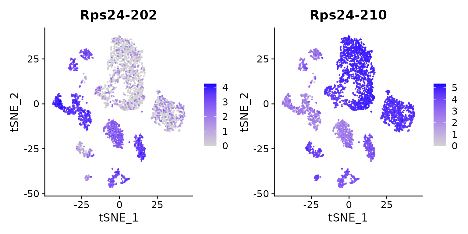
We see, that the isoforms are not specific for a single cell type, but for multiple. Still we see a striking difference, with a very pronounced expression of ‘Rps24-210’ in ‘T cell’, ‘B cell’, ‘macrophages’ and a small subcluster of ‘stromal cells’.
For later use we can save the final DTUrtle object to disk:
Session info
Computation time for this vignette:
#> Time difference of 2.50571 hours#> R version 3.6.2 (2019-12-12)
#> Platform: x86_64-pc-linux-gnu (64-bit)
#> Running under: Debian GNU/Linux 10 (buster)
#>
#> Matrix products: default
#> BLAS/LAPACK: /usr/lib/x86_64-linux-gnu/libopenblasp-r0.3.5.so
#>
#> locale:
#> [1] LC_CTYPE=en_US.UTF-8 LC_NUMERIC=C
#> [3] LC_TIME=en_US.UTF-8 LC_COLLATE=en_US.UTF-8
#> [5] LC_MONETARY=en_US.UTF-8 LC_MESSAGES=C
#> [7] LC_PAPER=en_US.UTF-8 LC_NAME=C
#> [9] LC_ADDRESS=C LC_TELEPHONE=C
#> [11] LC_MEASUREMENT=en_US.UTF-8 LC_IDENTIFICATION=C
#>
#> attached base packages:
#> [1] stats graphics grDevices utils datasets methods base
#>
#> other attached packages:
#> [1] Seurat_3.2.2 DTUrtle_1.0.2 sparseDRIMSeq_0.1.2
#>
#> loaded via a namespace (and not attached):
#> [1] reticulate_1.16 tidyselect_1.1.0
#> [3] RSQLite_2.2.1 AnnotationDbi_1.48.0
#> [5] htmlwidgets_1.5.2 grid_3.6.2
#> [7] BiocParallel_1.22.0 Rtsne_0.15
#> [9] munsell_0.5.0 codetools_0.2-16
#> [11] ragg_0.4.0 ica_1.0-2
#> [13] DT_0.16 future_1.19.1
#> [15] miniUI_0.1.1.1 colorspace_1.4-1
#> [17] Biobase_2.46.0 knitr_1.30
#> [19] rstudioapi_0.11 stats4_3.6.2
#> [21] ROCR_1.0-11 tensor_1.5
#> [23] listenv_0.8.0 labeling_0.4.2
#> [25] tximport_1.16.1 bbmle_1.0.23.1
#> [27] GenomeInfoDbData_1.2.2 polyclip_1.10-0
#> [29] bit64_4.0.5 farver_2.0.3
#> [31] pheatmap_1.0.12 rprojroot_1.3-2
#> [33] coda_0.19-4 Matrix.utils_0.9.8
#> [35] vctrs_0.3.4 generics_0.0.2
#> [37] xfun_0.18 biovizBase_1.34.1
#> [39] BiocFileCache_1.10.2 R6_2.4.1
#> [41] GenomeInfoDb_1.22.1 apeglm_1.8.0
#> [43] rsvd_1.0.3 locfit_1.5-9.4
#> [45] AnnotationFilter_1.10.0 bitops_1.0-6
#> [47] spatstat.utils_1.17-0 DelayedArray_0.12.3
#> [49] assertthat_0.2.1 promises_1.1.1
#> [51] scales_1.1.1 nnet_7.3-12
#> [53] gtable_0.3.0 globals_0.13.1
#> [55] goftest_1.2-2 ensembldb_2.10.2
#> [57] rlang_0.4.11 genefilter_1.68.0
#> [59] systemfonts_0.3.2 splines_3.6.2
#> [61] rtracklayer_1.46.0 lazyeval_0.2.2
#> [63] dichromat_2.0-0 formattable_0.2.0.1
#> [65] checkmate_2.0.0 yaml_2.2.1
#> [67] reshape2_1.4.4 abind_1.4-5
#> [69] crosstalk_1.1.0.1 GenomicFeatures_1.38.2
#> [71] backports_1.1.10 httpuv_1.5.4
#> [73] Hmisc_4.4-1 tools_3.6.2
#> [75] ggplot2_3.3.2 ellipsis_0.3.1
#> [77] RColorBrewer_1.1-2 BiocGenerics_0.32.0
#> [79] ggridges_0.5.2 Rcpp_1.0.5
#> [81] plyr_1.8.6 base64enc_0.1-3
#> [83] progress_1.2.2 zlibbioc_1.32.0
#> [85] purrr_0.3.4 RCurl_1.98-1.2
#> [87] prettyunits_1.1.1 rpart_4.1-15
#> [89] openssl_1.4.3 deldir_0.1-29
#> [91] pbapply_1.4-3 cowplot_1.1.0
#> [93] S4Vectors_0.24.4 zoo_1.8-8
#> [95] SummarizedExperiment_1.16.1 grr_0.9.5
#> [97] ggrepel_0.8.2 cluster_2.1.0
#> [99] fs_1.5.0 magrittr_2.0.1
#> [101] data.table_1.13.2 glmGamPoi_1.5.0
#> [103] lmtest_0.9-38 RANN_2.6.1
#> [105] mvtnorm_1.1-1 ProtGenerics_1.18.0
#> [107] fitdistrplus_1.1-1 matrixStats_0.57.0
#> [109] hms_0.5.3 patchwork_1.0.1
#> [111] mime_0.9 evaluate_0.14
#> [113] xtable_1.8-4 XML_3.99-0.3
#> [115] jpeg_0.1-8.1 emdbook_1.3.12
#> [117] IRanges_2.20.2 gridExtra_2.3
#> [119] compiler_3.6.2 biomaRt_2.42.1
#> [121] bdsmatrix_1.3-4 tibble_3.0.4
#> [123] KernSmooth_2.23-16 crayon_1.3.4
#> [125] htmltools_0.5.0 mgcv_1.8-31
#> [127] later_1.1.0.1 Formula_1.2-4
#> [129] tidyr_1.1.2 geneplotter_1.64.0
#> [131] DBI_1.1.0 dbplyr_1.4.4
#> [133] MASS_7.3-51.4 rappdirs_0.3.1
#> [135] Matrix_1.2-18 parallel_3.6.2
#> [137] Gviz_1.30.4 igraph_1.2.6
#> [139] GenomicRanges_1.38.0 pkgconfig_2.0.3
#> [141] pkgdown_1.6.1 GenomicAlignments_1.22.1
#> [143] foreign_0.8-72 numDeriv_2016.8-1.1
#> [145] plotly_4.9.2.1 annotate_1.64.0
#> [147] XVector_0.26.0 VariantAnnotation_1.32.0
#> [149] stringr_1.4.0 digest_0.6.26
#> [151] sctransform_0.3.1 RcppAnnoy_0.0.16
#> [153] spatstat.data_1.4-3 Biostrings_2.54.0
#> [155] rmarkdown_2.5 leiden_0.3.3
#> [157] htmlTable_2.1.0 uwot_0.1.8
#> [159] edgeR_3.28.1 curl_4.3
#> [161] shiny_1.5.0 Rsamtools_2.2.3
#> [163] lifecycle_1.0.1 nlme_3.1-142
#> [165] jsonlite_1.7.1 stageR_1.10.0
#> [167] BSgenome_1.54.0 askpass_1.1
#> [169] desc_1.2.0 viridisLite_0.3.0
#> [171] limma_3.42.2 pillar_1.4.6
#> [173] lattice_0.20-38 fastmap_1.0.1
#> [175] httr_1.4.2 survival_3.1-8
#> [177] glue_1.4.2 spatstat_1.64-1
#> [179] png_0.1-7 bit_4.0.4
#> [181] stringi_1.5.3 blob_1.2.1
#> [183] textshaping_0.1.2 DESeq2_1.33.1
#> [185] latticeExtra_0.6-29 memoise_1.1.0
#> [187] dplyr_1.0.2 irlba_2.3.3
#> [189] future.apply_1.6.0