Analysis of the Hoffman et al. human bulk RNA-seq data
Tobias Tekath
2021-11-18
Source:vignettes/Hoffman_human_bulk_analysis.Rmd
Hoffman_human_bulk_analysis.RmdThis vignette exemplifies the analysis of bulk RNA-seq data with DTUrtle. The data used in this vignette is publicly available as Bioproject PRJNA594939 and the used FASTQ-files can be downloaded from here. The corresponding publication from Hoffman et al. can be found here.
The following code shows an example of an DTUrtle workflow. Assume we have performed the pre-processing as described here and the R working directory is a newly created folder called dtu_results.
Setup
Load the DTUrtle package and set the BiocParallel parameter. It is recommended to perform computations in parallel, if possible.
library(DTUrtle)
#> Loading required package: sparseDRIMSeq
#> To cite DTUrtle in publications use:
#>
#>  Tobias Tekath, Martin Dugas.
#>  Differential transcript usage analysis
#>  of bulk and single-cell RNA-seq data with DTUrtle.
#>  Bioinformatics,
#>  2021.
#>  https://doi.org/10.1093/bioinformatics/btab629.
#>
#> Use citation(DTUrtle) for BibTeX information.
#use up to 10 cores for computation
biocpar <- BiocParallel::MulticoreParam(10)
Import and format data
We want to start by reading in our quantification counts, as well as a file specifying which transcript ID or name belongs to which gene ID or name.
Importing and processing GTF annotation (tx2gene)
To get this transcript to gene (tx2gene) mapping, we will utilize the already present Gencode annotation file gencode.v34.annotation.gtf. The import_gtf() function utilizes the a rtracklayer package and returns a transcript-level filtered version of the available data.
tx2gene <- import_gtf(gtf_file = "../gencode.v34.annotation.gtf")
head(tx2gene, n=3)
#>   seqnames start   end width strand source       type score phase
#> 1     chr1 11869 14409  2541      + HAVANA transcript    NA    NA
#> 2     chr1 12010 13670  1661      + HAVANA transcript    NA    NA
#> 3     chr1 14404 29570 15167      - HAVANA transcript    NA    NA
#>             gene_id     transcript_id                          gene_type
#> 1 ENSG00000223972.5 ENST00000456328.2 transcribed_unprocessed_pseudogene
#> 2 ENSG00000223972.5 ENST00000450305.2 transcribed_unprocessed_pseudogene
#> 3 ENSG00000227232.5 ENST00000488147.1             unprocessed_pseudogene
#>   gene_name                    transcript_type transcript_name level
#> 1   DDX11L1               processed_transcript     DDX11L1-202     2
#> 2   DDX11L1 transcribed_unprocessed_pseudogene     DDX11L1-201     2
#> 3    WASH7P             unprocessed_pseudogene      WASH7P-201     2
#>   transcript_support_level    hgnc_id   tag          havana_gene
#> 1                        1 HGNC:37102 basic OTTHUMG00000000961.1
#> 2                       NA HGNC:37102 basic OTTHUMG00000000961.1
#> 3                       NA HGNC:38034 basic OTTHUMG00000000958.1
#>      havana_transcript         ont protein_id ccdsid
#> 1 OTTHUMT00000362751.1        <NA>       <NA>   <NA>
#> 2 OTTHUMT00000002844.1 PGO:0000019       <NA>   <NA>
#> 3 OTTHUMT00000002839.1 PGO:0000005       <NA>   <NA>
There are a lot of columns present in the data frame, but at the moment we are mainly interested in the columns gene_id, gene_name, transcript_id and transcript_name.
As we want to use gene and transcript names as the main identifiers in our analysis (so we can directly say: Gene x is differential), we should ensure that each gene / transcript name maps only to a single gene / transcript id.
For this we can use the DTUrtle function one_to_one_mapping(), which checks if there are identifiers, which relate to the same name. If this is the case, the names (not the identifiers) are slightly altered by appending a number. If id_x and id_y both have the name ABC, the id_y name is altered to ABC_2 by default.
tx2gene$gene_name <- one_to_one_mapping(name = tx2gene$gene_name, id = tx2gene$gene_id)
#> Changed 78 names.
tx2gene$transcript_name <- one_to_one_mapping(name = tx2gene$transcript_name, id = tx2gene$transcript_id)
#> Changed 161 names.
We see that it was a good idea to ensure the one to one mapping, as many doublets have been corrected.
For the run_drimseq() tx2gene parameter, we need a data frame, where the first column specifies the transcript identifiers and the second column specifying the corresponding gene names. Rather than subsetting the data frame, a column reordering is proposed, so that additional data can still be used in further steps. DTUrtle makes sure to carry over additional data columns in the analysis steps. To reorder the columns of our tx2gene data frame, we can utilize the move_columns_to_front() functionality.
tx2gene <- move_columns_to_front(df = tx2gene, columns = c("transcript_name", "gene_name"))
head(tx2gene, n=5)
#>   transcript_name   gene_name seqnames start   end width strand  source
#> 1     DDX11L1-202     DDX11L1     chr1 11869 14409  2541      +  HAVANA
#> 2     DDX11L1-201     DDX11L1     chr1 12010 13670  1661      +  HAVANA
#> 3      WASH7P-201      WASH7P     chr1 14404 29570 15167      -  HAVANA
#> 4   MIR6859-1-201   MIR6859-1     chr1 17369 17436    68      - ENSEMBL
#> 5 MIR1302-2HG-202 MIR1302-2HG     chr1 29554 31097  1544      +  HAVANA
#>         type score phase           gene_id     transcript_id
#> 1 transcript    NA    NA ENSG00000223972.5 ENST00000456328.2
#> 2 transcript    NA    NA ENSG00000223972.5 ENST00000450305.2
#> 3 transcript    NA    NA ENSG00000227232.5 ENST00000488147.1
#> 4 transcript    NA    NA ENSG00000278267.1 ENST00000619216.1
#> 5 transcript    NA    NA ENSG00000243485.5 ENST00000473358.1
#>                            gene_type                    transcript_type level
#> 1 transcribed_unprocessed_pseudogene               processed_transcript     2
#> 2 transcribed_unprocessed_pseudogene transcribed_unprocessed_pseudogene     2
#> 3             unprocessed_pseudogene             unprocessed_pseudogene     2
#> 4                              miRNA                              miRNA     3
#> 5                             lncRNA                             lncRNA     2
#>   transcript_support_level    hgnc_id   tag          havana_gene
#> 1                        1 HGNC:37102 basic OTTHUMG00000000961.1
#> 2                       NA HGNC:37102 basic OTTHUMG00000000961.1
#> 3                       NA HGNC:38034 basic OTTHUMG00000000958.1
#> 4                       NA HGNC:50039 basic                 <NA>
#> 5                        5 HGNC:52482 basic OTTHUMG00000000959.1
#>      havana_transcript         ont protein_id ccdsid
#> 1 OTTHUMT00000362751.1        <NA>       <NA>   <NA>
#> 2 OTTHUMT00000002844.1 PGO:0000019       <NA>   <NA>
#> 3 OTTHUMT00000002839.1 PGO:0000005       <NA>   <NA>
#> 4                 <NA>        <NA>       <NA>   <NA>
#> 5 OTTHUMT00000002840.1        <NA>       <NA>   <NA>
This concludes the tx2gene formatting.
Reading in quantification data
The read-in of the quantification counts can be achieved with import_counts(), which uses the tximport package in the background. This function is able to parse the output of many different quantification tools. Advanced users might be able to tune parameters to parse arbitrary output files from currently not supported tools.
In the pre-processing vignette we quantified the counts with Salmon. The folder structure of the quantification results folder looks like this:
list.files("../salmon/")
#> [1] "bulk_D2hr_rep1" "bulk_D2hr_rep2" "bulk_D2hr_rep3" "bulk_EtOH_rep1"
#> [5] "bulk_EtOH_rep2" "bulk_EtOH_rep3" "index"
We will create a named files vector, pointing to the quant.sf file for each sample. The names help to differentiate the samples later on.
files <- Sys.glob("../salmon/bulk_*/quant.sf")
names(files) <- gsub(".*/","",gsub("/quant.sf","",files))
The files object looks like this:
#>                      bulk_D2hr_rep1                      bulk_D2hr_rep2
#> "../salmon/bulk_D2hr_rep1/quant.sf" "../salmon/bulk_D2hr_rep2/quant.sf"
#>                      bulk_D2hr_rep3                      bulk_EtOH_rep1
#> "../salmon/bulk_D2hr_rep3/quant.sf" "../salmon/bulk_EtOH_rep1/quant.sf"
#>                      bulk_EtOH_rep2                      bulk_EtOH_rep3
#> "../salmon/bulk_EtOH_rep2/quant.sf" "../salmon/bulk_EtOH_rep3/quant.sf"
The actual import will be performed with import_counts(). As we are analyzing bulk RNA-seq data, the raw counts should be scaled regarding transcript length and/or library size prior to analysis. DTUrtle will default to appropriate scaling schemes for your data. It is advised to provide a transcript to gene mapping for the tx2gene parameter, as then the tximport dtuScaledTPM scaling scheme can be applied. This schemes is especially designed for DTU analysis and scales by using the median transcript length among isoforms of a gene, and then the library size.
The raw counts from Salmon are named in regard to the transcript_id, thus we will provide an appropriate tx2gene parameter here. Downstream we want to use the transcript_name rather than the transcript_id, so we change the row names of the counts:
cts <- import_counts(files, type = "salmon", tx2gene=tx2gene[,c("transcript_id", "gene_name")])
#> Reading in 6 salmon runs.
#> Using 'dtuScaledTPM' for 'countsFromAbundance'.
#> reading in files with read_tsv
#> 1 2 3 4 5 6
rownames(cts) <- tx2gene$transcript_name[match(rownames(cts), tx2gene$transcript_id)]
dim(cts)
#> [1] 227201      6
There are ~227k features left for the six samples. Please note, that in contrast to the single-cell workflow utilizing combine_to_matrix(), these counts also include features with no expression. These will be filtered out by the DTUrtle filtering step in run_drimseq().
Sample metadata
Finally, we need a sample metadata data frame, specifying which sample belongs to which comparison group. This table is also convenient to store and carry over additional metadata.
If such a table is not already present, it can be easily prepared:
pd <- data.frame("id"=colnames(cts),
                 "group"=c(rep("Dex2hr",3), rep("EtOH",3)),
                 stringsAsFactors = FALSE)
head(pd, n=5)
#>               id  group
#> 1 bulk_D2hr_rep1 Dex2hr
#> 2 bulk_D2hr_rep2 Dex2hr
#> 3 bulk_D2hr_rep3 Dex2hr
#> 4 bulk_EtOH_rep1   EtOH
#> 5 bulk_EtOH_rep2   EtOH
DTU analysis
We have prepared all necessary data to perform the differentially transcript usage (DTU) analysis. DTUrtle only needs two simple commands to perform it. Please be aware that these steps are the most compute intensive and, depending on your data, might take some time to complete. It is recommended to parallelize the computations with the BBPARAM parameter, if applicable.
First, we want to set-up and perform the statistical analysis with DRIMSeq, a DTU specialized statistical framework utilizing a Dirichlet-multinomial model. This can be done with the run_drimseq() command. We use the previously imported data as parameters, specifying which column in the cell metadata data frame contains ids and which the group information we want. We should also specify which of the groups should be compared (if there are more than two) and in which order. The order given in the cond_levels parameter also specifies the comparison formula.
dturtle <- run_drimseq(counts = cts, tx2gene = tx2gene, pd=pd, id_col = "id",
                    cond_col = "group", cond_levels = c("Dex2hr", "EtOH"), filtering_strategy = "bulk",
                    BPPARAM = biocpar)
#> Using tx2gene columns:
#>  transcript_name ---> 'feature_id'
#>  gene_name ---> 'gene_id'
#>
#> Comparing in 'group': 'Dex2hr' vs 'EtOH'
#>
#> Proceed with cells/samples:
#> Dex2hr   EtOH
#>      3      3
#>
#> Filtering...
#>
  |
  |                                                                      |   0%
  |
  |=======                                                               |  10%
  |
  |==============                                                        |  20%
  |
  |=====================                                                 |  30%
  |
  |============================                                          |  40%
  |
  |===================================                                   |  50%
  |
  |==========================================                            |  60%
  |
  |=================================================                     |  70%
  |
  |========================================================              |  80%
  |
  |===============================================================       |  90%
  |
  |======================================================================| 100%
#> Retain 52805 of 152311 features.
#> Removed 99506 features.
#>
#> Performing statistical tests...
#> * Calculating mean gene expression..
#> * Estimating common precision..
#> ! Using common_precision = 13.1556 as prec_init !
#> * Estimating genewise precision..
#> ! Using loess fit as a shrinkage factor !
#> * Fitting the DM model..
#>    Using the one way approach.
#> * Fitting the BB model..
#>    Using the one way approach.
#> * Fitting the DM model..
#>    Using the one way approach.
#> * Calculating likelihood ratio statistics..
#> * Fitting the BB model..
#>    Using the one way approach.
#> * Calculating likelihood ratio statistics..
As in all statistical procedures, it is of favor to perform as few tests as possible but as much tests as necessary, to maintain a high statistical power. This is achieved by filtering the data to remove inherently uninteresting items, for example very lowly expressed genes or features. DTUrtle includes a powerful and customizable filtering functionality for this task, which is an optimized version of the dmFilter() function of the DRIMSeq package.
Above we used a predefined filtering strategy for bulk data, requiring that features contribute at least 5% of the total expression in at least 50% of the cells of the smallest group. Also the total gene expression must be 5 or more for at least 50% of the samples of the smallest group. Additionally, all genes are filtered, which only have a single transcript left, as they can not be analyzed in DTU analysis. The filtering options can be extended or altered by the user.
dturtle$used_filtering_options
#> $DRIM
#> $DRIM$min_samps_gene_expr
#> [1] 1.5
#>
#> $DRIM$min_samps_feature_expr
#> [1] 0
#>
#> $DRIM$min_samps_feature_prop
#> [1] 1.5
#>
#> $DRIM$min_gene_expr
#> [1] 5
#>
#> $DRIM$min_feature_expr
#> [1] 0
#>
#> $DRIM$min_feature_prop
#> [1] 0.05
#>
#> $DRIM$run_gene_twice
#> [1] TRUE
The resulting dturtle object will be used as our main results object, storing all necessary and interesting data of the analysis. It is a simple and easy-accessible list, which can be easily extended / altered by the user. By default three different meta data tables are generated:
-
meta_table_gene: Contains gene level meta data. -
meta_table_tx: Contains transcript level meta data. -
meta_table_sample: Contains sample level meta data (as the createdpddata frame)
These meta data tables are used in for visualization purposes and can be extended by the user.
dturtle$meta_table_gene[1:5,1:5]
#>              gene exp_in exp_in_Dex2hr exp_in_EtOH seqnames
#> A1BG-AS1 A1BG-AS1      1             1           1    chr19
#> A2M-AS1   A2M-AS1      1             1           1    chr12
#> A2ML1       A2ML1      1             1           1    chr12
#> A4GALT     A4GALT      1             1           1    chr22
#> AAAS         AAAS      1             1           1    chr12
As proposed in Love et al. (2018), we will use a two-stage statistical testing procedure together with a post-hoc filtering on the standard deviations in proportions (posthoc_and_stager()). We will use stageR to determine genes, that show a overall significant change in transcript proportions. For these significant genes, we will try to pinpoint specific transcripts, which significantly drive this overall change. As a result, we will have a list of significant genes (genes showing the overall change) and a list of significant transcripts (one or more transcripts of the significant genes). Please note, that not every significant gene does have one or more significant transcripts. It is not always possible to attribute the overall change in proportions to single transcripts. These two list of significant items are computed and corrected against a overall false discovery rate (OFDR).
Additionally, we will apply a post-hoc filtering scheme to improve the targeted OFDR control level. The filtering strategy will discard transcripts, which standard deviation of the proportion per cell/sample is below the specified threshold. For example by setting posthoc=0.1, we will exclude all transcripts, which proportional expression (in regard to the total gene expression) deviates by less than 0.1 between cells. This filtering step should mostly exclude ‘uninteresting’ transcripts, which would not have been called as significant either way.
dturtle <- posthoc_and_stager(dturtle = dturtle, ofdr = 0.05, posthoc = 0.1)
#> Posthoc filtered 38192 features.
#> The returned adjusted p-values are based on a stage-wise testing approach and are only valid for the provided target OFDR level of 5%. If a different target OFDR level is of interest,the entire adjustment should be re-run.
#> Found 294 significant genes with 146 significant transcripts (OFDR: 0.05)
The dturtle object now contains additional elements, including the lists of significant genes and significant transcripts.
head(dturtle$sig_gene)
#> [1] "ABCC8"      "ABHD5"      "AC011603.3" "AC012063.1" "AC015813.1"
#> [6] "AC090809.1"
head(dturtle$sig_tx)
#>            ABHD5       AC011603.3       AC015813.1       AC090809.1
#>      "ABHD5-208" "AC011603.3-203" "AC015813.1-201" "AC090809.1-203"
#>       AC093323.1       AC093323.1
#> "AC093323.1-202" "AC093323.1-204"
(optional) DGE analysis
Alongside a DTU analysis, a DGE analysis might be of interest for your research question. DTUrtle offers a basic DGE calling workflow for bulk and single-cell RNA-seq data via DESeq2.
To utilize this workflow, we should re-scale our imported counts. The transcript-level count matrix has been scaled for the DTU analysis, but for a DGE analysis un-normalized counts should be used (as DESeq2 normalizes internally). We can simply re-import the count data, by providing the already defined files object to the DGE analysis specific function import_dge_counts(). This function will make sure that the counts are imported but not scaled and also summarizes to gene-level.
Our files object looks like this:
head(files)
#>                      bulk_D2hr_rep1                      bulk_D2hr_rep2
#> "../salmon/bulk_D2hr_rep1/quant.sf" "../salmon/bulk_D2hr_rep2/quant.sf"
#>                      bulk_D2hr_rep3                      bulk_EtOH_rep1
#> "../salmon/bulk_D2hr_rep3/quant.sf" "../salmon/bulk_EtOH_rep1/quant.sf"
#>                      bulk_EtOH_rep2                      bulk_EtOH_rep3
#> "../salmon/bulk_EtOH_rep2/quant.sf" "../salmon/bulk_EtOH_rep3/quant.sf"
We re-import the files with the same parameters as before:
cts_dge <- import_dge_counts(files, type="salmon", tx2gene=tx2gene[,c("transcript_id", "gene_name")])
#> Reading in 6 salmon runs.
#> reading in files with read_tsv
#> 1 2 3 4 5 6
#> summarizing abundance
#> summarizing counts
#> summarizing length
With this data, we can perform the DGE analysis with DESeq2 with the DTUrtle function run_deseq2(). DESeq2 is one of the gold-standard tools for DGE calling in bulk RNA-seq data and showed very good performance for single-cell data in multiple benchmarks. The DESeq2 vignette recommends adjusting some parameters for DGE analysis of single-cell data - DTUrtle incorporates these recommendations and adjusts the specific parameters based on the provided dge_calling_strategy().
After the DESeq2 DGE analysis, the estimated log2 fold changes are shrunken (preferably with apeglm) - to provide a secondary ranking variable beside the statistical significance. If a shrinkage with apeglm is performed, run_deseq2() defaults to also compute s-values rather than adjusted p-values. The underlying hypothesis for s-values and (standard) p-values differs slightly, with s-values hypothesis being presumably preferential in a real biological context. Far more information about all these topics can be found in the excellent DESeq2 vignette and the associated publications.
run_deseq2() will tell the user, if one or more advised packages are missing. It is strongly advised to follow these recommendations.
dturtle$dge_analysis <- run_deseq2(counts = cts_dge, pd = pd, id_col = "id",
                                   cond_col = "group", cond_levels = c("Dex2hr", "EtOH"),
                                   lfc_threshold = 1, sig_threshold = 0.01, dge_calling_strategy = "bulk",
                                   BPPARAM = biocpar)
#>
#> Comparing in 'group': 'Dex2hr' vs 'EtOH'
#>
#> Proceed with cells/samples:
#> Dex2hr   EtOH
#>      3      3
#> using counts and average transcript lengths from tximport
#> estimating size factors
#> using 'avgTxLength' from assays(dds), correcting for library size
#> estimating dispersions
#> gene-wise dispersion estimates: 10 workers
#> mean-dispersion relationship
#> final dispersion estimates, fitting model and testing: 10 workers
#> using 'apeglm' for LFC shrinkage. If used in published research, please cite:
#>     Zhu, A., Ibrahim, J.G., Love, M.I. (2018) Heavy-tailed prior distributions for
#>     sequence count data: removing the noise and preserving large differences.
#>     Bioinformatics. https://doi.org/10.1093/bioinformatics/bty895
#> computing FSOS 'false sign or small' s-values (T=1)
#> Found 211 significant DEGs.
#>      Over-expressed: 197
#>      Under-expressed: 14
We provided a log2 fold change threshold of 1 (on log2 scale), thus preferring an effect size of 2x or more. The output of run_deseq2() is a list, containing various elements (see run_deseq2()’s description). This result list can easily added to an existing DTUrtle object, as shown above.
We can now identify genes which show both a DGE and DTU signal:
dtu_dge_genes <- intersect(dturtle$sig_gene, dturtle$dge_analysis$results_sig$gene)
length(dtu_dge_genes)
#> [1] 14
Result aggregation and visualization
The DTUrtle package contains multiple visualization options, enabling an in-depth inspection.
DTU table creation
We will start by aggregating the analysis results to a data frame with create_dtu_table(). This function is highly flexible and allows aggregation of gene or transcript level metadata in various ways. By default some useful information are included in the dtu table, in this example we further specify to include the seqnames column of the gene level metadata (which contains chromosome information) as well as the maximal expressed in ratio from the transcript level metadata.
dturtle <- create_dtu_table(dturtle = dturtle, add_gene_metadata = list("chromosome"="seqnames"),
                               add_tx_metadata = list("tx_expr_in_max" = c("exp_in", max)))
head(dturtle$dtu_table, n=5)
#>               gene_ID  gene_qvalue minimal_tx_qvalue number_tx
#> SMOX             SMOX 1.614207e-03      1.000000e+00         3
#> LINC00608   LINC00608 3.205655e-20      5.610821e-17         3
#> GAB3             GAB3 1.168830e-03      2.791593e-02         3
#> AL445524.2 AL445524.2 2.505591e-03      4.799752e-02         3
#> B3GAT2         B3GAT2 3.454037e-02      0.000000e+00         2
#>            number_significant_tx max(Dex2hr-EtOH) chromosome tx_expr_in_max
#> SMOX                           0        0.9368511      chr20      0.5000000
#> LINC00608                      1       -0.8749399       chr2      1.0000000
#> GAB3                           1        0.8514122       chrX      0.6666667
#> AL445524.2                     1        0.8160855       chr1      0.6666667
#> B3GAT2                         2       -0.7861951       chr6      0.6666667
The column definitions are as follows:
- “gene_ID”: Gene name or identifier used for the analysis.
- “gene_qvalue”: Multiple testing corrected p-value (a.k.a. q-value) comparing all transcripts together between the two groups (“gene level”).
- “minimal_tx_qvalue”: The minimal multiple testing corrected p-value from comparing all transcripts individually between the two groups (“transcript level”). I.e. the q-value of the most significant transcript.
- “number_tx”: The number of analyzed transcripts for the specific gene.
- “number_significant_tx”: The number of significant transcripts from the ‘transcript level’ analysis.
- “max(Dex2hr-EtOH)”: Maximal proportional difference between the two groups (Dex2hr vs EtOH). E.g. one transcript of ‘SMOX’ is ~94% more expressed in ‘Dex2hr’ cells compared to ‘EtOH’ cells.
- “chromosome”: the chromosome the gene resides on.
- “tx_expr_in_max”: The fraction of cells, the most expressed transcript is expressed in. “Expressed in” is defined as expression>0.
This table is our basis for creating an interactive HTML-table of the results.
Proportion barplot
As a first visualization option we will create a barplot of the proportions of each transcript per sample. We can use the function plot_proportion_barplot() for this task, which also adds the mean proportion fit per subgroup to the plot (by default as a red line).
As an example, we will create the plot for the gene TSC22D3 (a Glucocorticoid-Induced Leucine Zipper), which is one of the significant genes found in the analysis. Additionally, it is identified in Hoffman et al. as one of the Dexamethasone / Glucocorticoid Receptor target genes, which also shows differential expression already after 2 hours of Dex treatment.
We will optionally provide the gene_id for TSC22D3, which is stored in the column gene_id.1 of dturtle$meta_table_gene.
temp <- plot_proportion_barplot(dturtle = dturtle, genes = "TSC22D3", meta_gene_id = "gene_id.1")
#> Creating 1 plots:
temp$TSC22D3
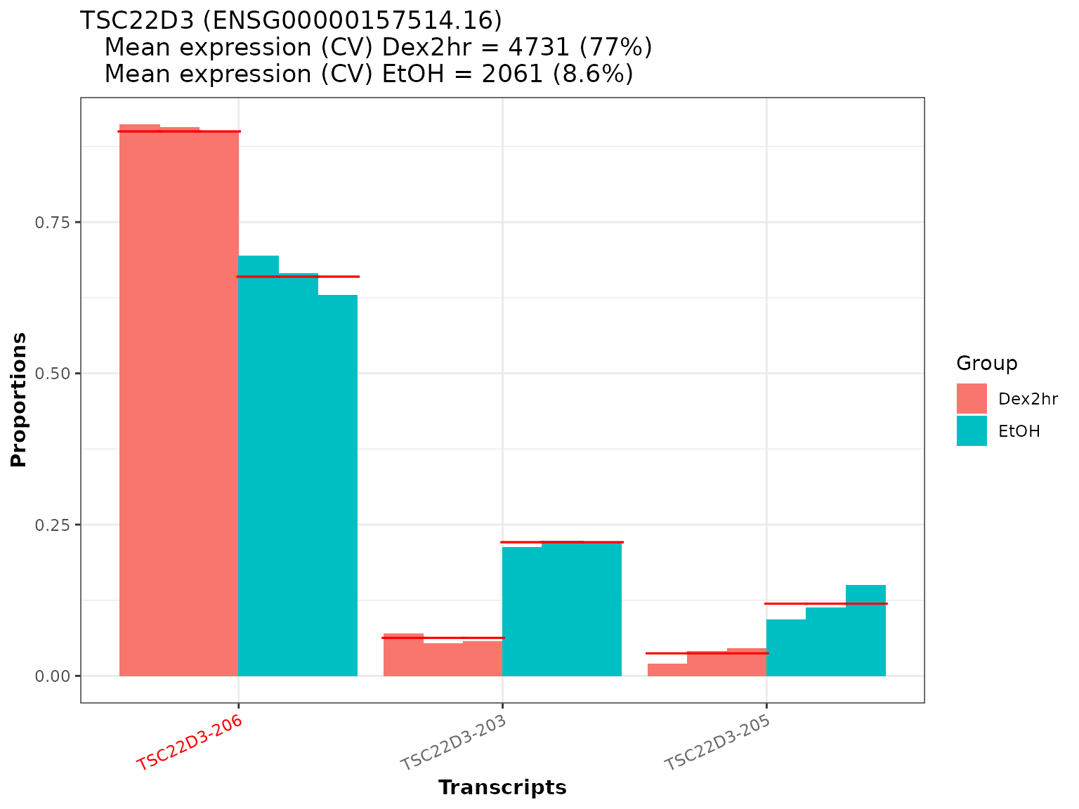
We see, that there are striking proportional differences for the three transcripts of TSC22D3. Due to Dexamethasone treatment, there seems to be a shift to almost exclusive expression of TSC22D3-206. This transcript has also been identified as a significant transcript in the analysis (as the name is marked in red). From the top annotation we can also see, that the mean total expression of TSC22D3 is higher in the Dex2hr group (as expected) - but also the coefficient of variation (CV) is higher, indicating a higher variance between the samples.
For the interactive HTML-table we would need to save the images to disk (in the to-be-created sub folder “images” of the current working directory). There is also a convenience option, to directly add the file paths to the dtu_table. As multiple plots are created, we can provide a BiocParallel object to speed up the creation. If no specific genes are provided, all significant genes will be plotted.
dturtle <- plot_proportion_barplot(dturtle = dturtle,
                                   meta_gene_id = "gene_id.1",
                                   savepath = "images",
                                   add_to_table = "barplot",
                                   BPPARAM = biocpar)
#> Creating 294 plots:
#>
  |
  |                                                                      |   0%
  |
  |=======                                                               |  10%
  |
  |==============                                                        |  20%
  |
  |=====================                                                 |  30%
  |
  |============================                                          |  40%
  |
  |===================================                                   |  50%
  |
  |==========================================                            |  60%
  |
  |=================================================                     |  70%
  |
  |========================================================              |  80%
  |
  |===============================================================       |  90%
  |
|======================================================================| 100%head(dturtle$dtu_table$barplot) #> [1] "images/SMOX_barplot.png" "images/LINC00608_barplot.png" #> [3] "images/GAB3_barplot.png" "images/AL445524.2_barplot.png" #> [5] "images/B3GAT2_barplot.png" "images/SCARF1_barplot.png" head(list.files("./images/")) #> [1] "ABCC8_barplot.png" "ABHD5_barplot.png" "AC011603.3_barplot.png" #> [4] "AC012063.1_barplot.png" "AC015813.1_barplot.png" "AC090809.1_barplot.png"
Proportion heatmap
A different visualization option is a heatmap, where additional meta data can be displayed alongside the transcript proportions (plot_proportion_pheatmap()). This visualization uses the pheatmap package, the user can specify any of the available parameters to customize the results.
temp <- plot_proportion_pheatmap(dturtle = dturtle, genes = "TSC22D3",
                                 include_expression = TRUE, treeheight_col=20)
#> Creating 1 plots:
temp$TSC22D3
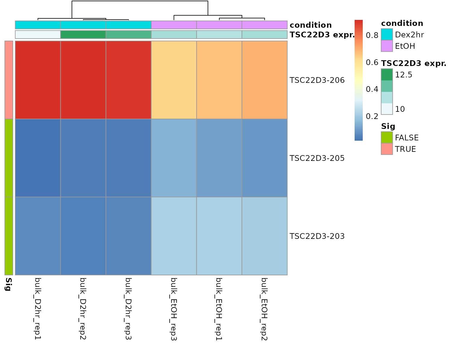
By default, row and column annotations are added. This plot helps to examine the transcript composition of groups of cells. We can see a quite uniform expression pattern between the two conditions. From the column annotation we can see, that the TSC22D3 total expression in the sample bulk_D2hr_rep1 is quite lower than in the rest.
Again, we can save the plots to disk and add them to the dtu_table:
dturtle <- plot_proportion_pheatmap(dturtle = dturtle,
                                    include_expression = TRUE,
                                    treeheight_col=20,
                                    savepath = "images",
                                    add_to_table = "pheatmap",
                                    BPPARAM = biocpar)
#> Creating 294 plots:
#>
  |
  |                                                                      |   0%
  |
  |=======                                                               |  10%
  |
  |==============                                                        |  20%
  |
  |=====================                                                 |  30%
  |
  |============================                                          |  40%
  |
  |===================================                                   |  50%
  |
  |==========================================                            |  60%
  |
  |=================================================                     |  70%
  |
  |========================================================              |  80%
  |
  |===============================================================       |  90%
  |
|======================================================================| 100%head(dturtle$dtu_table$pheatmap) #> [1] "images/SMOX_pheatmap.png" "images/LINC00608_pheatmap.png" #> [3] "images/GAB3_pheatmap.png" "images/AL445524.2_pheatmap.png" #> [5] "images/B3GAT2_pheatmap.png" "images/SCARF1_pheatmap.png" head(list.files("./images/")) #> [1] "ABCC8_barplot.png" "ABCC8_pheatmap.png" #> [3] "ABHD5_barplot.png" "ABHD5_pheatmap.png" #> [5] "AC011603.3_barplot.png" "AC011603.3_pheatmap.png"
Transcript overview
Until now, we looked at the different transcripts as abstract entities. Alongside proportional differences, the actual difference in the exon-intron structure of transcripts is of great importance for many research questions. This structure can be visualized with the plot_transcripts_view() functionality of DTUrtle.
This visualization is based on the Gviz package and needs a path to a GTF file (or a read-in object). In Import and format data we already imported a GTF file. This was subset to transcript-level (via the import_gtf() function), thus this is not sufficient for the visualization. We can reuse the actual GTF file though, which should in general match with the one used for the tx2gene data frame.
As we have ensured the one_to_one mapping in Import and format data and potentially renamed some genes, we should specify the one_to_one parameter in this call.
plot_transcripts_view(dturtle = dturtle,
                              genes = "TSC22D3",
                              gtf = "../gencode.v34.annotation.gtf",
                              genome = 'hg38',
                              one_to_one = TRUE)
#>
#> Importing gtf file from disk.
#>
#> Performing one to one mapping in gtf
#>
#> Found gtf GRanges for 1 of 1 provided genes.
#>
#> Fetching ideogram tracks ...
#> Creating 1 plots:

#> $TSC22D3
#> $TSC22D3$chrX
#> Ideogram track 'chrX' for chromosome X of the hg38 genome
#>
#> $TSC22D3$OverlayTrack
#> OverlayTrack 'OverlayTrack' containing 2 subtracks
#>
#> $TSC22D3$OverlayTrack
#> OverlayTrack 'OverlayTrack' containing 2 subtracks
#>
#> $TSC22D3$OverlayTrack
#> OverlayTrack 'OverlayTrack' containing 2 subtracks
#>
#> $TSC22D3$titles
#> An object of class "ImageMap"
#> Slot "coords":
#>              x1       y1   x2        y2
#> chrX          6 120.0000 58.2  186.8141
#> OverlayTrack  6 186.8141 58.2  506.5427
#> OverlayTrack  6 506.5427 58.2  826.2714
#> OverlayTrack  6 826.2714 58.2 1146.0000
#>
#> Slot "tags":
#> $title
#>           chrX   OverlayTrack   OverlayTrack   OverlayTrack
#>         "chrX" "OverlayTrack" "OverlayTrack" "OverlayTrack"
This visualization shows the structure of the transcripts of TSC22D3. The significant transcript (TSC22D3-206) is quite different to the other mainly expressed transcript (TSC22D3-203). TSC22D3-206 has a different first exon than TSC22D3-203, whose first exon is quite far away from the conserved transcript body. The arrows on the right side indicate the mean fitted proportional change in the comparison groups, thus showing a over-expression of TSC22D3-206 in Dex2hr compared to EtOH.
The areas between exons indicate intron sequences, which have been compressed in this representation to highlight the exon structure. Only consensus introns are compressed to a defined minimal size. This can be turned off with reduce_introns=FALSE or alternatively reduced introns can be highlighted by setting a colorful reduce_introns_fill.
Analogous as before, we can save plots to disk and add them to the dtu_table:
dturtle <- plot_transcripts_view(dturtle = dturtle,
                                 gtf = "../gencode.v34.annotation.gtf",
                                 genome = 'hg38',
                                 one_to_one = TRUE,
                                 savepath = "images",
                                 add_to_table = "transcript_view",
                                 BPPARAM = biocpar)
#>
#> Importing gtf file from disk.
#>
#> Performing one to one mapping in gtf
#>
#> Found gtf GRanges for 294 of 294 provided genes.
#>
#> Fetching ideogram tracks ...
#> Creating 294 plots:
#>
  |
  |                                                                      |   0%
  |
  |=======                                                               |  10%
  |
  |==============                                                        |  20%
  |
  |=====================                                                 |  30%
  |
  |============================                                          |  40%
  |
  |===================================                                   |  50%
  |
  |==========================================                            |  60%
  |
  |=================================================                     |  70%
  |
  |========================================================              |  80%
  |
  |===============================================================       |  90%
  |
|======================================================================| 100%head(dturtle$dtu_table$transcript_view) #> [1] "images/SMOX_transcripts.png" "images/LINC00608_transcripts.png" #> [3] "images/GAB3_transcripts.png" "images/AL445524.2_transcripts.png" #> [5] "images/B3GAT2_transcripts.png" "images/SCARF1_transcripts.png" head(list.files("./images/")) #> [1] "ABCC8_barplot.png" "ABCC8_pheatmap.png" "ABCC8_transcripts.png" #> [4] "ABHD5_barplot.png" "ABHD5_pheatmap.png" "ABHD5_transcripts.png"
Visualize DTU table
The dturtle$dtu_table is now ready to be visualized as an interactive HTML-table. Please note, that it is optional to add any plots or additional columns to the table. Thus the visualization will work directly after calling create_dtu_table().
The dtu_table object looks like this:
head(dturtle$dtu_table)
#>               gene_ID  gene_qvalue minimal_tx_qvalue number_tx
#> SMOX             SMOX 1.614207e-03      1.000000e+00         3
#> LINC00608   LINC00608 3.205655e-20      5.610821e-17         3
#> GAB3             GAB3 1.168830e-03      2.791593e-02         3
#> AL445524.2 AL445524.2 2.505591e-03      4.799752e-02         3
#> B3GAT2         B3GAT2 3.454037e-02      0.000000e+00         2
#> SCARF1         SCARF1 2.421844e-03      1.066113e-04         3
#>            number_significant_tx max(Dex2hr-EtOH) chromosome tx_expr_in_max
#> SMOX                           0        0.9368511      chr20      0.5000000
#> LINC00608                      1       -0.8749399       chr2      1.0000000
#> GAB3                           1        0.8514122       chrX      0.6666667
#> AL445524.2                     1        0.8160855       chr1      0.6666667
#> B3GAT2                         2       -0.7861951       chr6      0.6666667
#> SCARF1                         2        0.7627478      chr17      0.8333333
#>                                  barplot                       pheatmap
#> SMOX             images/SMOX_barplot.png       images/SMOX_pheatmap.png
#> LINC00608   images/LINC00608_barplot.png  images/LINC00608_pheatmap.png
#> GAB3             images/GAB3_barplot.png       images/GAB3_pheatmap.png
#> AL445524.2 images/AL445524.2_barplot.png images/AL445524.2_pheatmap.png
#> B3GAT2         images/B3GAT2_barplot.png     images/B3GAT2_pheatmap.png
#> SCARF1         images/SCARF1_barplot.png     images/SCARF1_pheatmap.png
#>                              transcript_view
#> SMOX             images/SMOX_transcripts.png
#> LINC00608   images/LINC00608_transcripts.png
#> GAB3             images/GAB3_transcripts.png
#> AL445524.2 images/AL445524.2_transcripts.png
#> B3GAT2         images/B3GAT2_transcripts.png
#> SCARF1         images/SCARF1_transcripts.png
Before creating the actual table, we can optionally define column formatter functions, which color the specified columns. The coloring might help with to quickly dissect the results.
DTUrtle come with some pre-defined column formatter functions (for p-values and percentages), other formatter functions from the formattable package can also be used. Advanced users might also define their own functions.
We create a named list, linking column names to formatter functions:
column_formatter_list <- list(
      "gene_qvalue" = table_pval_tile("white", "orange", digits = 3),
      "minimal_tx_qvalue" = table_pval_tile("white", "orange", digits = 3),
      "number_tx" = formattable::color_tile('white', "lightblue"),
      "number_significant_tx" = formattable::color_tile('white', "lightblue"),
      "max(Dex2hr-EtOH)" = table_percentage_bar('lightgreen', "#FF9999", digits=2),
      "tx_expr_in_max" = table_percentage_bar('white', "lightblue", color_break = 0, digits=2))
This column_formatter_list is subsequently provided to plot_dtu_table():
plot_dtu_table(dturtle = dturtle, savepath = "my_results.html",
               column_formatters = column_formatter_list)
Note: ️As seen above, the paths to the plots are relative. Please make sure that the saving directory in
plot_dtu_table()is correctly set and the plots are reachable from that directory with the given path.The links in the following example are just for demonstration purposes and do not work!
For later use we can save the final DTUrtle object to disk:
saveRDS(dturtle, "./dturtle_res.RDS")
Session info
Computation time for this vignette:
#> Time difference of 17.99346 mins#> R version 3.6.2 (2019-12-12)
#> Platform: x86_64-pc-linux-gnu (64-bit)
#> Running under: Debian GNU/Linux 10 (buster)
#>
#> Matrix products: default
#> BLAS/LAPACK: /usr/lib/x86_64-linux-gnu/libopenblasp-r0.3.5.so
#>
#> locale:
#> [1] LC_CTYPE=en_US.UTF-8 LC_NUMERIC=C
#> [3] LC_TIME=en_US.UTF-8 LC_COLLATE=en_US.UTF-8
#> [5] LC_MONETARY=en_US.UTF-8 LC_MESSAGES=C
#> [7] LC_PAPER=en_US.UTF-8 LC_NAME=C
#> [9] LC_ADDRESS=C LC_TELEPHONE=C
#> [11] LC_MEASUREMENT=en_US.UTF-8 LC_IDENTIFICATION=C
#>
#> attached base packages:
#> [1] stats graphics grDevices utils datasets methods base
#>
#> other attached packages:
#> [1] DTUrtle_1.0.2 sparseDRIMSeq_0.1.2
#>
#> loaded via a namespace (and not attached):
#> [1] backports_1.1.10 Hmisc_4.4-1
#> [3] BiocFileCache_1.10.2 systemfonts_0.3.2
#> [5] plyr_1.8.6 lazyeval_0.2.2
#> [7] splines_3.6.2 crosstalk_1.1.0.1
#> [9] BiocParallel_1.22.0 GenomeInfoDb_1.22.1
#> [11] ggplot2_3.3.2 digest_0.6.26
#> [13] ensembldb_2.10.2 stageR_1.10.0
#> [15] htmltools_0.5.0 formattable_0.2.0.1
#> [17] magrittr_2.0.1 checkmate_2.0.0
#> [19] memoise_1.1.0 BSgenome_1.54.0
#> [21] cluster_2.1.0 limma_3.42.2
#> [23] Biostrings_2.54.0 readr_1.4.0
#> [25] annotate_1.64.0 matrixStats_0.57.0
#> [27] askpass_1.1 bdsmatrix_1.3-4
#> [29] pkgdown_1.6.1 prettyunits_1.1.1
#> [31] jpeg_0.1-8.1 colorspace_1.4-1
#> [33] blob_1.2.1 rappdirs_0.3.1
#> [35] apeglm_1.8.0 textshaping_0.1.2
#> [37] xfun_0.18 dplyr_1.0.2
#> [39] crayon_1.3.4 RCurl_1.98-1.2
#> [41] jsonlite_1.7.1 tximport_1.16.1
#> [43] genefilter_1.68.0 VariantAnnotation_1.32.0
#> [45] survival_3.1-8 glue_1.4.2
#> [47] gtable_0.3.0 zlibbioc_1.32.0
#> [49] XVector_0.26.0 DelayedArray_0.12.3
#> [51] BiocGenerics_0.32.0 scales_1.1.1
#> [53] pheatmap_1.0.12 mvtnorm_1.1-1
#> [55] DBI_1.1.0 edgeR_3.28.1
#> [57] Rcpp_1.0.5 xtable_1.8-4
#> [59] progress_1.2.2 emdbook_1.3.12
#> [61] htmlTable_2.1.0 foreign_0.8-72
#> [63] bit_4.0.4 Formula_1.2-4
#> [65] DT_0.16 stats4_3.6.2
#> [67] htmlwidgets_1.5.2 httr_1.4.2
#> [69] RColorBrewer_1.1-2 ellipsis_0.3.1
#> [71] pkgconfig_2.0.3 XML_3.99-0.3
#> [73] farver_2.0.3 Gviz_1.30.4
#> [75] nnet_7.3-12 dbplyr_1.4.4
#> [77] locfit_1.5-9.4 tidyselect_1.1.0
#> [79] labeling_0.4.2 rlang_0.4.11
#> [81] reshape2_1.4.4 AnnotationDbi_1.48.0
#> [83] munsell_0.5.0 tools_3.6.2
#> [85] generics_0.0.2 RSQLite_2.2.1
#> [87] evaluate_0.14 stringr_1.4.0
#> [89] yaml_2.2.1 ragg_0.4.0
#> [91] knitr_1.30 bit64_4.0.5
#> [93] fs_1.5.0 purrr_0.3.4
#> [95] AnnotationFilter_1.10.0 mime_0.9
#> [97] grr_0.9.5 biomaRt_2.42.1
#> [99] compiler_3.6.2 rstudioapi_0.11
#> [101] curl_4.3 png_0.1-7
#> [103] tibble_3.0.4 geneplotter_1.64.0
#> [105] stringi_1.5.3 GenomicFeatures_1.38.2
#> [107] desc_1.2.0 lattice_0.20-38
#> [109] ProtGenerics_1.18.0 Matrix_1.2-18
#> [111] vctrs_0.3.4 pillar_1.4.6
#> [113] lifecycle_1.0.1 data.table_1.13.2
#> [115] bitops_1.0-6 Matrix.utils_0.9.8
#> [117] rtracklayer_1.46.0 GenomicRanges_1.38.0
#> [119] R6_2.4.1 latticeExtra_0.6-29
#> [121] gridExtra_2.3 IRanges_2.20.2
#> [123] dichromat_2.0-0 MASS_7.3-51.4
#> [125] assertthat_0.2.1 SummarizedExperiment_1.16.1
#> [127] openssl_1.4.3 DESeq2_1.33.1
#> [129] rprojroot_1.3-2 GenomicAlignments_1.22.1
#> [131] Rsamtools_2.2.3 S4Vectors_0.24.4
#> [133] GenomeInfoDbData_1.2.2 parallel_3.6.2
#> [135] hms_0.5.3 grid_3.6.2
#> [137] rpart_4.1-15 coda_0.19-4
#> [139] rmarkdown_2.5 biovizBase_1.34.1
#> [141] bbmle_1.0.23.1 numDeriv_2016.8-1.1
#> [143] Biobase_2.46.0 base64enc_0.1-3